[11]:

import astropy.units as u
import matplotlib.pyplot as plt
import numpy as np
from astropy.visualization import quantity_support

from mocksipipeline.detector.response import SpectrogramChannel, ThinFilmFilter

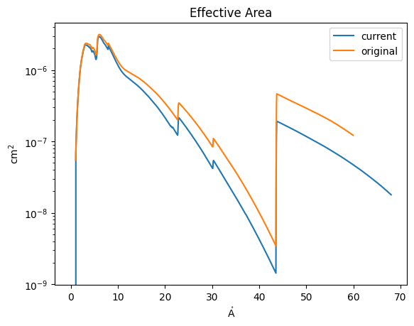
Effective Area–Old versus Current Effective Area Model#

This notebook compares the current versus original conception of the effective area curves for the dispersed channel. “Original” refers to the conception as used for the modeling in the proposal

[15]:

al_filter = ThinFilmFilter(elements='Al', thickness=150*u.nm, xrt_table='Chantler')

[16]:

spec_chan = SpectrogramChannel(1, al_filter)

[18]:

with quantity_support():
    plt.plot(spec_chan.wavelength, spec_chan.effective_area, label='current')
    plt.plot(spec_chan._data['wave'], spec_chan._data['effarea'], label='original')
plt.yscale('log')
plt.legend()
plt.title('Effective Area')

[18]:

Text(0.5, 1.0, 'Effective Area')

../_images/reports_effective-area-comparison_4_1.png

[21]:

with quantity_support():
    plt.plot(spec_chan.wavelength, spec_chan.filter_transmission, label='current')
    plt.plot(spec_chan._data['wave'], spec_chan._data['filter'], label='original')
plt.title('Filter Transmission')
plt.legend()

[21]:

<matplotlib.legend.Legend at 0x17eb88910>

../_images/reports_effective-area-comparison_5_1.png

Notably, the grating efficiency in our current model now includes a Au-Cr base plate.

[23]:

with quantity_support():
    plt.plot(spec_chan.wavelength, spec_chan.grating_efficiency, label='current')
    plt.plot(spec_chan._data['wave'], spec_chan._data['grating'], label='original')
plt.yscale('log')
plt.title('Grating Efficiency')
plt.legend()

[23]:

<matplotlib.legend.Legend at 0x17ed22ac0>

../_images/reports_effective-area-comparison_7_1.png

[ ]: