Modeling Wavelength Response of the MOXSI Detectors#
[83]:
import sys
import copy

import astropy.units as u
import astropy.constants as const
import astropy.io.fits
import astropy.wcs
from ndcube import NDCube
from astropy.visualization import quantity_support
import numpy as np
import matplotlib.pyplot as plt
from scipy.interpolate import interp1d
from aiapy.response import Channel as AIAChannel

from roentgen.absorption import Material, Response

sys.path.append('../simulation_pipeline/detector/')
from response import Channel, SpectrogramChannel
Response Function Comparison#
[2]:
selected_filters = [
    'Be_thin',
    'Be_med',
    'Be_thick',
    'Al_poly',
]
chan_filename = '../simulation_pipeline/data/MOXSI_effarea.genx'
pinholes = [Channel(f, chan_filename) for f in selected_filters]
dispersed_orders = [SpectrogramChannel(o, chan_filename) for o in [0,1,3]]
[50]:
for p in pinholes:
    print(f'{p.name}: {p._data["filter_desc"]}')
Be_thin: 9 micron Be filter / XRT thin Be - no support
Be_med: 30 micron Be filter / XRT med Be - no support
Be_thick: 300 micron Be filter / XRT thick Be - no support
Al_poly: 1.25 micron Al filter * 2.5 micron Poly / XRT Al-Poly
[77]:
fig = plt.figure(figsize=(14,7))
ax = fig.add_subplot(111)
#ax2 = ax.twiny()
for p in pinholes:
    ax.plot(p.wavelength, p.wavelength_response, label=p.name)
    #energy = const.h * const.c / p.wavelength
    #ax2.plot(energy.to('keV'), p.wavelength_response)
for d in dispersed_orders:
    ax.plot(d.wavelength, d.wavelength_response, label=d.name, ls='--')
ax.legend()
ax.set_yscale('log')
ax.set_ylim(1e-9,0.03)
#ax.set_xlim(p.wavelength[[0,-1]].to_value('angstrom'))

energy_ticks = lambda x: [f"{(const.h * const.c / (_x*u.angstrom)).to_value('keV'):.2f}" for _x in x]

#energy_even = np.logspace(-1,1,10) * u.keV

#new_tick_locations = (const.h * const.c / energy_even).to_value('angstrom')

new_tick_locations = range(1,70,10)

ax2 = ax.twiny()
ax2.set_xlim(ax.get_xlim())
ax2.set_xticks(new_tick_locations)
ax2.set_xticklabels(energy_ticks(new_tick_locations));

ax.set_ylabel(f'Wavelength response [{p.wavelength_response.unit}]')
ax.set_xlabel(f'Wavelength [{p.wavelength.unit}]')
ax2.set_xlabel('Energy [keV]');

[52]:
def read_cube(filename, hdu=0):
    with astropy.io.fits.open(filename) as hdul:
        data = hdul[hdu].data
        header = hdul[hdu].header
        header.pop('KEYCOMMENTS', None)
        wcs = astropy.wcs.WCS(header=header)
        spec_cube = NDCube(data, wcs=wcs, meta=header, unit=header.get('BUNIT', None))
    return spec_cube
[54]:
spectral_cube = read_cube('../simulation_pipeline/spectral-cube-example.fits', hdu=1)
[64]:
def convolve_with_response(cube, channel):
    """
    Convolve spectral cube with wavelength response to convert spectra to instrument units.

    Parameters
    ----------
    cube : `ndcube.NDCube`
    channel : `Channel`

    Return
    ------
    : `ndcube.NDCube`
        Spectral cube in detector units convolved with instrument response
    """
    CDELT_SPACE = 5.66 * u.arcsec / u.pix
    CDELT_WAVE = 55 * u.milliangstrom / u.pix
    # FIXME: this should go in the Channel object
    plate_scale = CDELT_SPACE * CDELT_SPACE * u.pix
    # Interpolate wavelength response to wavelength array of spectral cube
    # NOTE: should this be done in reverse?
    wavelength = cube.axis_world_coords(0)[0].to_value('Angstrom')
    f_response = interp1d(channel.wavelength.to_value('Angstrom'),
                          channel.wavelength_response.to_value(),
                          bounds_error=False,
                          fill_value=0.0,)  # Response is 0 outside of the response range
    response = u.Quantity(f_response(wavelength), channel.wavelength_response.unit)
    response *= plate_scale
    response *= CDELT_WAVE * u.pix

    # Multiply by spectral cube
    data = (cube.data.T * cube.unit * response).T.sum(axis=0)

    meta = copy.deepcopy(cube.meta)
    meta['channel_name'] = channel.name

    return NDCube(data.to('ct pix-1 s-1'), wcs=cube[0].wcs, meta=meta)
[69]:
pinhole_images = []
for p in pinholes:
    pinhole_images.append(convolve_with_response(spectral_cube, p))
WARNING: VerifyWarning: Keyword name 'channel_name' is greater than 8 characters or contains characters not allowed by the FITS standard; a HIERARCH card will be created. [astropy.io.fits.card]
[78]:
from astropy.visualization import ImageNormalize, LogStretch
import sunpy.map
[80]:
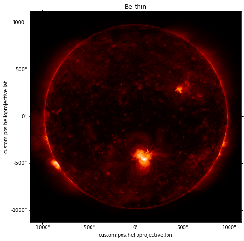
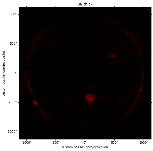
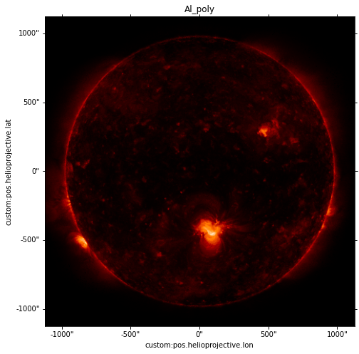
norm = ImageNormalize(vmin=0,vmax=50,stretch=LogStretch())
for pi in pinhole_images:
    fig = plt.figure(figsize=(8,8))
    ax = fig.add_subplot(111, projection=pi.wcs)
    pi.plot(axes=ax,norm=norm,cmap='hinodexrt')
    ax.set_title(pi.meta['channel_name'])

[84]:
aia_channels = [AIAChannel(c) for c in [94,131,171,193,211,335]*u.angstrom]
[87]:
aia_channels[0].wavelength_response()
[87]:
[ ]:
aia_images = [convolve_with_response(spectral_cube, ac) for ac in aia_channels]
Dispersed Channel#
Look first at our current approach to modeling wave response
[3]:
chan = SpectrogramChannel(1, '../simulation_pipeline/data/MOXSI_effarea.genx')
[24]:
for c in chan._instrument_data['SAVEGEN0']:
    print(c['CHANNEL'])
    print('--------------')
    print('Filter:',c['FILTER_DESC'])
    print('Detector:',c['DET_DESC'])
    print('\n')
MOXSI_S0
--------------
Filter: 100 nm of Al based on conversation with Amir 11/11/20
Detector: Assumed based on transimission of Si


MOXSI_S1
--------------
Filter: 100 nm of Al based on conversation with Amir 11/11/20
Detector: Assumed based on transimission of Si


MOXSI_S3
--------------
Filter: 100 nm of Al based on conversation with Amir 11/11/20
Detector: Assumed based on transimission of Si


MOXSI_S5
--------------
Filter: 100 nm of Al based on conversation with Amir 11/11/20
Detector: Assumed based on transimission of Si


Be_thin
--------------
Filter: 9 micron Be filter / XRT thin Be - no support
Detector: Assumed based on transimission of Si


Be_med
--------------
Filter: 30 micron Be filter / XRT med Be - no support
Detector: Assumed based on transimission of Si


Be_thick
--------------
Filter: 300 micron Be filter / XRT thick Be - no support
Detector: Assumed based on transimission of Si


Al_poly
--------------
Filter: 1.25 micron Al filter * 2.5 micron Poly / XRT Al-Poly
Detector: Assumed based on transimission of Si


Al_med
--------------
Filter: 12.5 micron Al filter / XRT Al med - no support
Detector: Assumed based on transimission of Si


C_poly
--------------
Filter: 6 micron C filter * 2.5 micron poly / XRT C-poly
Detector: Assumed based on transimission of Si


Ti_poly
--------------
Filter: 6 micron C filter * 2.5 micron poly / XRT C-poly
Detector: Assumed based on transimission of Si
[25]:
al = Material('Al', 100*u.nm)
[26]:
energy = const.h * const.c / chan.wavelength
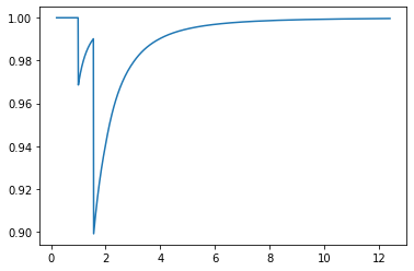
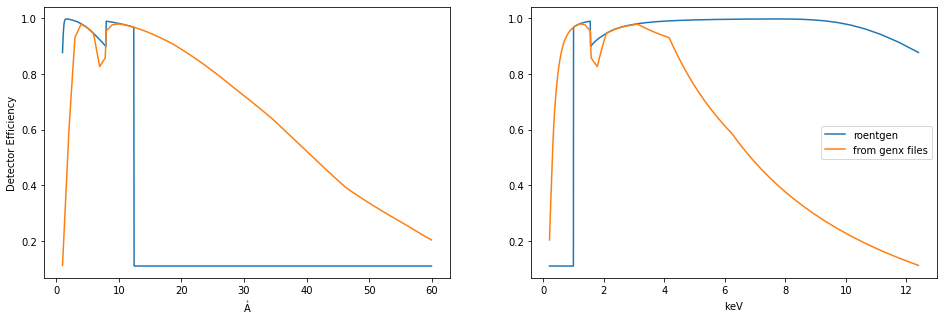
Clearly there is some additional component here that causes the drop off starting at \(\approx15\mathrm{\mathring{A}}\)
[73]:
energy.to('keV')
[73]:
[76]:
plt.plot(energy.to('keV'), al.transmission(energy))
plt.xlim()
[76]:
[<matplotlib.lines.Line2D at 0x7fdc812d5b50>]
[45]:
plt.figure(figsize=(16,5))
plt.subplot(121)
with quantity_support():
    plt.plot(wavelength, al.transmission(energy), label=f'{al.name}')
    plt.plot(wavelength, chan.filter_transmission, label='from genx files')
plt.ylabel(f'Filter Transmission')
plt.subplot(122)
with quantity_support():
    plt.plot(energy.to('keV'), al.transmission(energy), label=f'{al.name}')
    plt.plot(energy.to('keV'), chan.filter_transmission, label='from genx files')
plt.legend()
[45]:
<matplotlib.legend.Legend at 0x7fdc800f9ee0>

What is the assumed thickness here? Are there other materials? Shouldn’t this be absorption rather than transmission?
[67]:
si = Material('Si', 500*u.micron)
[68]:
plt.figure(figsize=(16,5))
plt.subplot(121)
with quantity_support():
    plt.plot(wavelength, si.absorption(energy), label=f'{si.name}')
    plt.plot(wavelength, chan.detector_efficiency, label='from genx files')
plt.ylabel(f'Detector Efficiency')
plt.subplot(122)
with quantity_support():
    plt.plot(energy.to('keV'), si.absorption(energy), label=f'{si.name}')
    plt.plot(energy.to('keV'), chan.detector_efficiency, label='from genx files')
plt.legend()
[68]:
<matplotlib.legend.Legend at 0x7fdc9f283e80>

Try using the roentgen.material.Response object
[69]:
materials = [
    Material('al', 100*u.nm),
]
detector = Material('si', 500*u.micron)
response = Response(materials, detector)
[70]:
chan.detector_efficiency * chan.filter_transmission
[70]:
[71]:
plt.figure(figsize=(16,5))
plt.subplot(121)
with quantity_support():
    plt.plot(wavelength, response.response(energy), label=f'roentgen')
    plt.plot(wavelength, chan.detector_efficiency * chan.filter_transmission, label='from genx files')
plt.ylabel(f'Detector Efficiency')
plt.subplot(122)
with quantity_support():
    plt.plot(energy.to('keV'), response.response(energy), label=f'roentgen')
    plt.plot(energy.to('keV'), chan.detector_efficiency * chan.filter_transmission, label='from genx files')
plt.legend()
[71]:
<matplotlib.legend.Legend at 0x7fdc9ec58070>
Pinhole Images#
Questions#
What materials are in the optical path of our detector? Currently, just assuming Al (for dispersed image)
What are the materials for the pinhole filters? (is proposal correct?)
What are the associated thicknesses of each of these components?
When it comes to modeling the detector, should this be absorption?
What is the quantum efficiency of the detector?
QE is probability of observing photon?
Or is it the conversion from photon to electron different?
Or different active involvement of the detector?
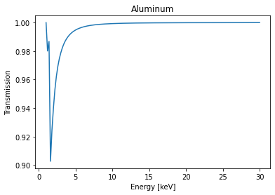
[81]:
al = Material('Al', 100 * u.nm)
energy = u.Quantity(np.arange(.99, 30, 0.2), 'keV')

plt.plot(energy, al.transmission(energy))
plt.ylabel('Transmission')
plt.xlabel('Energy [' + str(energy.unit) + ']')
plt.title(al.name)
[81]:
Text(0.5, 1.0, 'Aluminum')
[84]:
(const.h * const.c / (50*u.eV)).to('Angstrom')
[84]:
[86]:
(const.h * const.c).to('keV angstrom')
[86]:
Sandbox#
[48]:
import astropy.units as u
import astropy.constants as const
import matplotlib.pyplot as plt
import numpy as np
from roentgen.absorption import Material

al = Material('Al',100*u.nm)

wavelength = np.arange(1,60,1) * u .angstrom
energy = const.h * const.c / wavelength

transmission = al.transmission(energy)
mac = al.mass_attenuation_coefficient.func(energy)
[52]:
mac
[52]:
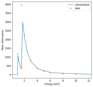
[50]:
plt.figure(figsize=(6,6))
plt.subplot(111)
plt.plot(energy.to('keV'),mac, label='interpolated')
plt.plot(al.mass_attenuation_coefficient.energy, al.mass_attenuation_coefficient.data, marker='*', ls='', label='data')
plt.xlim(energy[[-1,0]].to('keV').value)
plt.ylabel('Mass attenuation')
plt.xlabel('Energy [keV]')
plt.legend()
[50]:
<matplotlib.legend.Legend at 0x7fae20bb2eb0>
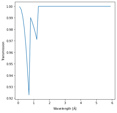
[54]:
plt.figure(figsize=(6,6))
plt.subplot(111)
plt.plot(wavelength.to('nm'), transmission)
plt.xlabel('Wavelength [$\mathrm{\mathring{A}}$]')
plt.ylabel('Transmission')
[54]:
Text(0, 0.5, 'Transmission')
[59]:
(100 * u.nm).to('um')
[59]:
[57]:
wavelength.to('nm')
[57]:
[ ]: