Flare Flux Budget#
[1]:
import pathlib
import numpy as np
import astropy.units as u
import matplotlib.pyplot as plt
from astropy.visualization import quantity_support, ImageNormalize, LogStretch, AsymmetricPercentileInterval
from astropy.convolution import convolve, Gaussian1DKernel
import ndcube
from ndcube.extra_coords import QuantityTableCoordinate
import fiasco
import aiapy.response

from fiasco.io import Parser
from synthesizAR.instruments import InstrumentDEM

from mocksipipeline.physics.spectral import get_spectral_tables
from mocksipipeline.detector.response import SpectrogramChannel, convolve_with_response, ThinFilmFilter

%matplotlib inline
Flux Budget for Flare DEMs#
Set up flare DEM from CHIANTI
[2]:
def dem_table_to_ndcube(dem_table):
    temperature = dem_table['temperature_bin_center']
    em = dem_table['dem']*np.gradient(temperature, edge_order=2)
    tab_coord = QuantityTableCoordinate(temperature,
                                        names='temperature',
                                        physical_types='phys.temperature')
    return ndcube.NDCube(em, wcs=tab_coord.wcs, meta=dem_table.meta)
[3]:
tab_flare = Parser('flare.dem', ascii_dbase_root='/Users/wtbarnes/ssw/packages/chianti/dbase/').parse()
dem_flare = dem_table_to_ndcube(tab_flare)
tab_flare_ext = Parser('flare_ext.dem', ascii_dbase_root='/Users/wtbarnes/ssw/packages/chianti/dbase/').parse()
dem_flare_ext = dem_table_to_ndcube(tab_flare_ext)
tab_ar = Parser('active_region.dem', ascii_dbase_root='/Users/wtbarnes/ssw/packages/chianti/dbase/').parse()
dem_ar = dem_table_to_ndcube(tab_ar)
[4]:
plt.figure(figsize=(10, 5))
with quantity_support():
    plt.plot(dem_flare.axis_world_coords(0)[0], dem_flare.data*dem_flare.unit, label='flare.dem')
    plt.plot(dem_flare_ext.axis_world_coords(0)[0], dem_flare_ext.data*dem_flare_ext.unit, label='flare_ext.dem')
    plt.plot(dem_ar.axis_world_coords(0)[0], dem_ar.data*dem_ar.unit, label='active_region.dem')
plt.xscale('log')
plt.yscale('log')
plt.legend()
[4]:
<matplotlib.legend.Legend at 0x1040c4b20>

Get spectra
[5]:
spec_tables = get_spectral_tables()
WARNING: UnitsWarning: The unit 'Angstrom' has been deprecated in the VOUnit standard. Suggested: 0.1nm. [astropy.units.format.utils]
WARNING: AstropyDeprecationWarning: The truth value of a Quantity is ambiguous. In the future this will raise a ValueError. [astropy.units.quantity]
Set up instrument response
[6]:
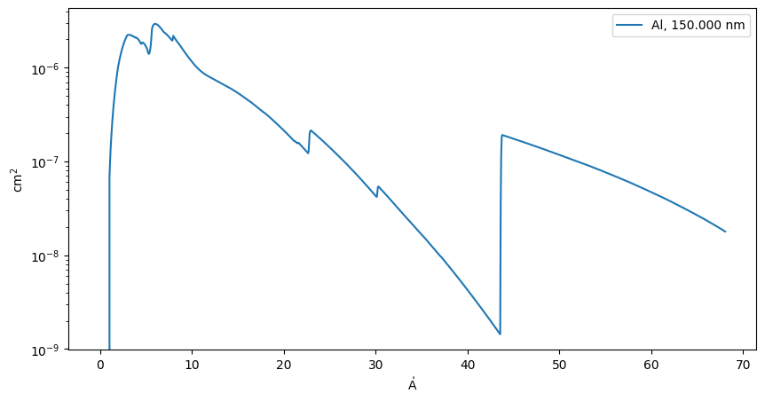
al_filter = ThinFilmFilter(elements='Al', thickness=150*u.nm, xrt_table='Chantler')
[7]:
chan = SpectrogramChannel(1, al_filter)
[8]:
plt.figure(figsize=(10,5))
with quantity_support():
    plt.plot(chan.wavelength, chan.effective_area, label=chan.filter_label)
plt.yscale('log')
plt.legend()
/Users/wtbarnes/mambaforge/envs/mocksipipeline/lib/python3.9/site-packages/astropy/units/quantity.py:626: RuntimeWarning: divide by zero encountered in divide
  result = super().__array_ufunc__(function, method, *arrays, **kwargs)
/Users/wtbarnes/mambaforge/envs/mocksipipeline/lib/python3.9/site-packages/astropy/units/quantity.py:626: RuntimeWarning: divide by zero encountered in divide
  result = super().__array_ufunc__(function, method, *arrays, **kwargs)
[8]:
<matplotlib.legend.Legend at 0x28898b490>
Compute spectrum
[9]:
intensity_flare = InstrumentDEM.calculate_intensity(dem_flare, spec_tables['sun_coronal_1992_feldman_ext_all'], {})
intensity_flare_ext = InstrumentDEM.calculate_intensity(dem_flare_ext, spec_tables['sun_coronal_1992_feldman_ext_all'], {})
intensity_ar = InstrumentDEM.calculate_intensity(dem_ar, spec_tables['sun_coronal_1992_feldman_ext_all'], {})
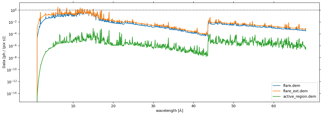
flux_flare = convolve_with_response(intensity_flare, chan, electrons=False, include_gain=False)
flux_flare_ext = convolve_with_response(intensity_flare_ext, chan, electrons=False, include_gain=False)
flux_ar = convolve_with_response(intensity_ar, chan, electrons=False, include_gain=False)
WARNING: UnitsWarning: The unit 'Angstrom' has been deprecated in the VOUnit standard. Suggested: 0.1nm. [astropy.units.format.utils]
[10]:
fig = plt.figure(figsize=(15,5))
ax = fig.add_subplot(projection=flux_flare)
flux_flare.plot(axes=ax, label='flare.dem')
flux_flare_ext.plot(axes=ax, label='flare_ext.dem')
flux_ar.plot(axes=ax, label='active_region.dem')
ax.set_yscale('log')
ax.axhline(y=1, color='k', ls=':')
ax.legend()
[10]:
<matplotlib.legend.Legend at 0x288b5f850>
[11]:
fig = plt.figure(figsize=(15,5))
ax = fig.add_subplot(projection=flux_flare)
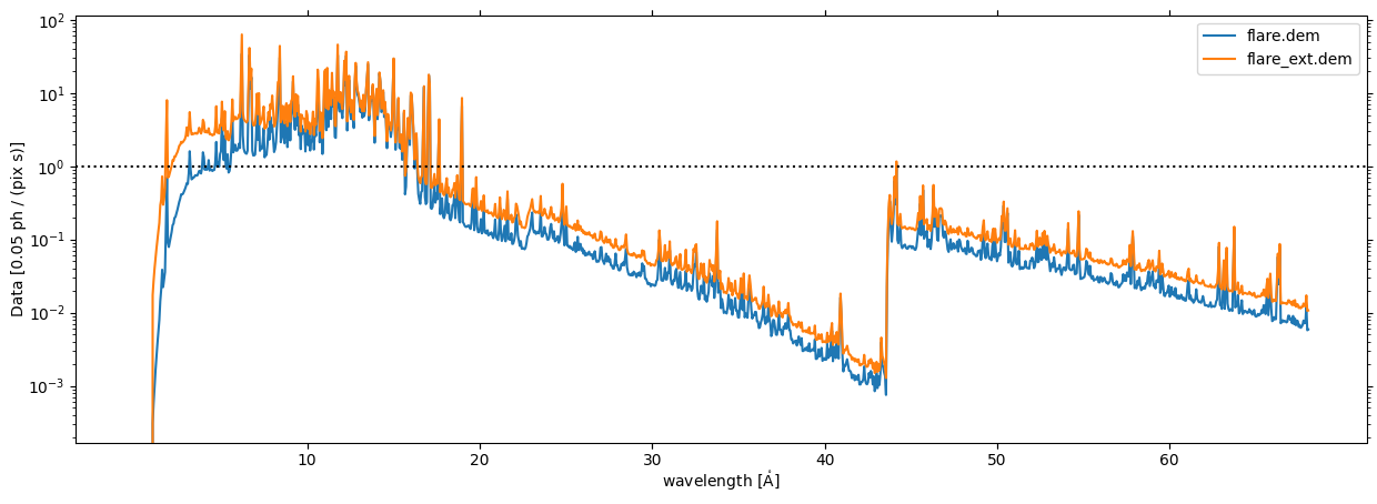
flux_flare.plot(axes=ax, label='flare.dem', data_unit=u.ph / u.pix / (20 * u.s))
flux_flare_ext.plot(axes=ax, label='flare_ext.dem', data_unit=u.ph / u.pix / (20 * u.s))
ax.set_yscale('log')
ax.axhline(y=1, color='k', ls=':')
ax.legend()
WARNING: UnitsWarning: The unit 'Angstrom' has been deprecated in the VOUnit standard. Suggested: 0.1nm. [astropy.units.format.utils]
[11]:
<matplotlib.legend.Legend at 0x288d6eb50>
[12]:
fig = plt.figure(figsize=(15,5))
ax = fig.add_subplot(projection=flux_flare)
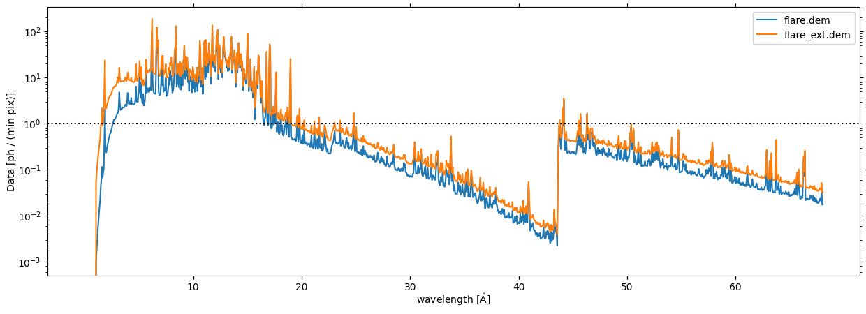
flux_flare.plot(axes=ax, label='flare.dem', data_unit=u.ph / u.pix / u.minute)
flux_flare_ext.plot(axes=ax, label='flare_ext.dem', data_unit=u.ph / u.pix / u.minute)
ax.set_yscale('log')
ax.axhline(y=1, color='k', ls=':')
ax.legend()
WARNING: UnitsWarning: The unit 'Angstrom' has been deprecated in the VOUnit standard. Suggested: 0.1nm. [astropy.units.format.utils]
[12]:
<matplotlib.legend.Legend at 0x28a2938e0>
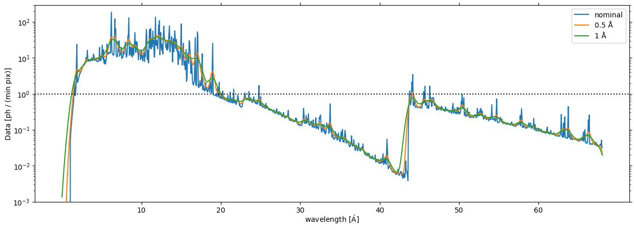
Effects on Spectral Resolution#
[13]:
def degrade_spectra(spec, resolution):
    std = resolution / (2*np.sqrt(2*np.log(2)))  # FWHM is 0.5 so convert to sigma using W = 2\sqrt{2\ln2}\sigma
    std_eff = (std / chan.spectral_resolution).to_value('pix')  # Scale sigma by bin width
    kernel = Gaussian1DKernel(std_eff)
    data_smooth = convolve(spec.data, kernel)
    return ndcube.NDCube(data_smooth, wcs=spec.wcs, meta=spec.meta, unit=spec.unit)
[14]:
flux_05 = degrade_spectra(flux_flare_ext, 0.5*u.angstrom)
flux_10 = degrade_spectra(flux_flare_ext, 1*u.angstrom)
[15]:
fig = plt.figure(figsize=(15,5))
ax = fig.add_subplot(projection=flux_flare_ext)
flux_flare_ext.plot(axes=ax, label='nominal', data_unit=u.ph / u.pix / u.minute)
flux_05.plot(axes=ax, label='0.5 Å', data_unit=u.ph / u.pix / u.minute)
flux_10.plot(axes=ax, label='1 Å', data_unit=u.ph / u.pix / u.minute)
ax.set_yscale('log')
ax.set_ylim(1e-3, 3e2)
ax.axhline(y=1, color='k', ls=':')
ax.legend()
WARNING: UnitsWarning: The unit 'Angstrom' has been deprecated in the VOUnit standard. Suggested: 0.1nm. [astropy.units.format.utils]
[15]:
<matplotlib.legend.Legend at 0x28a445af0>
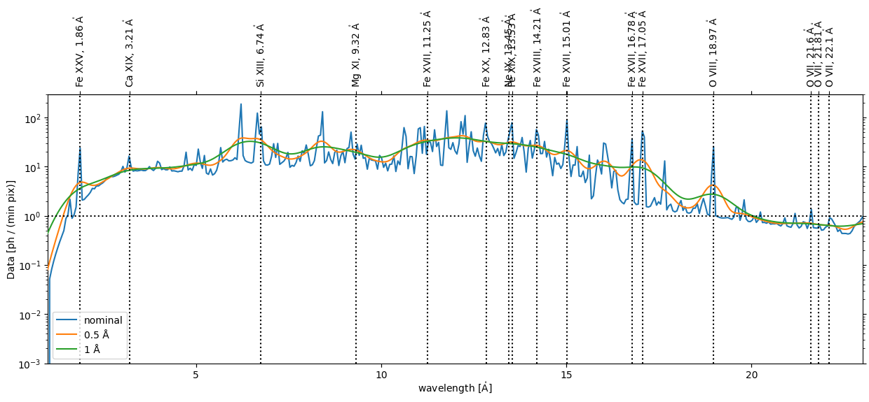
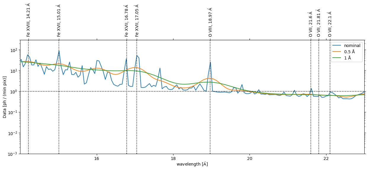
Looking at particular lines
[16]:
line_ids = [
    ('Fe XVIII',14.21*u.angstrom),  # also targeted by MaGIXS
    ('Fe XVII', 15.01*u.angstrom),  # also targeted by MaGIXS
    ('Fe XVII', 16.78*u.AA),
    ('Fe XVII', 17.05*u.AA),
    ('O VII', 21.60*u.angstrom),  # also targeted by MaGIXS
    ('O VII', 21.81*u.angstrom),
    ('O VII', 22.10*u.AA),
    ('O VIII', 18.97*u.angstrom),  # also targeted by MaGIXS
    ('Fe XXV', 1.86*u.AA),
    ('Ca XIX', 3.21*u.AA),
    ('Si XIII', 6.74*u.AA),
    ('Mg XI', 9.32*u.AA),
    ('Fe XVII', 11.25*u.AA),
    ('Fe XX', 12.83*u.AA),
    ('Ne IX', 13.45*u.AA),
    ('Fe XIX', 13.53*u.AA),
    ('C VI', 33.73*u.AA),
    ('C V', 40.27*u.AA),
    ('Si XII', 44.16*u.AA),
    ('Si XI', 49.18*u.AA),
]
[17]:
def add_line_ids_to_axis(ax, line_ids, rotation=90):
    for ion,line in line_ids:
        ax.axvline(x=ax.wcs.world_to_pixel(line), ls=':', color='k',)
    ax2 = ax.secondary_xaxis('top')
    ax2.set_xticks(ax.wcs.world_to_pixel(u.Quantity([l for _,l in line_ids])),
                   labels=[f'{ion}, {line.to_string(format="latex_inline")}' for ion,line in line_ids],
                   rotation=rotation,
                   horizontalalignment='center',
                   #verticalalignment='center'
                  )
[18]:
fig = plt.figure(figsize=(15,5))
ax = fig.add_subplot(projection=flux_flare_ext)
flux_flare_ext.plot(axes=ax, label='nominal', data_unit=u.ph / u.pix / u.minute)
flux_05.plot(axes=ax, label='0.5 Å', data_unit=u.ph / u.pix / u.minute)
flux_10.plot(axes=ax, label='1 Å', data_unit=u.ph / u.pix / u.minute)
ax.set_yscale('log')
ax.set_ylim(1e-3, 3e2)
ax.axhline(y=1, color='k', ls=':')
ax.legend()
add_line_ids_to_axis(ax, line_ids)
#ax.set_xlim(ax.wcs.world_to_pixel([14,23]*u.angstrom))
WARNING: UnitsWarning: The unit 'Angstrom' has been deprecated in the VOUnit standard. Suggested: 0.1nm. [astropy.units.format.utils]
[19]:
fig = plt.figure(figsize=(15,5))
ax = fig.add_subplot(projection=flux_flare_ext)
flux_flare_ext.plot(axes=ax, label='nominal', data_unit=u.ph / u.pix / u.minute)
flux_05.plot(axes=ax, label='0.5 Å', data_unit=u.ph / u.pix / u.minute)
flux_10.plot(axes=ax, label='1 Å', data_unit=u.ph / u.pix / u.minute)
ax.set_yscale('log')
ax.set_ylim(1e-3, 3e2)
ax.axhline(y=1, color='k', ls=':')
add_line_ids_to_axis(ax, line_ids)
ax.set_xlim(ax.wcs.world_to_pixel([1,23]*u.angstrom))
ax.legend(loc=3)
WARNING: UnitsWarning: The unit 'Angstrom' has been deprecated in the VOUnit standard. Suggested: 0.1nm. [astropy.units.format.utils]
[19]:
<matplotlib.legend.Legend at 0x28b46c370>
[20]:
fig = plt.figure(figsize=(15,5))
ax = fig.add_subplot(projection=flux_flare_ext)
flux_flare_ext.plot(axes=ax, label='nominal', data_unit=u.ph / u.pix / u.minute)
flux_05.plot(axes=ax, label='0.5 Å', data_unit=u.ph / u.pix / u.minute)
flux_10.plot(axes=ax, label='1 Å', data_unit=u.ph / u.pix / u.minute)
ax.set_yscale('log')
ax.set_ylim(1e-3, 3e2)
ax.axhline(y=1, color='k', ls=':')
ax.legend()
add_line_ids_to_axis(ax, line_ids)
ax.set_xlim(ax.wcs.world_to_pixel([14,23]*u.angstrom))
WARNING: UnitsWarning: The unit 'Angstrom' has been deprecated in the VOUnit standard. Suggested: 0.1nm. [astropy.units.format.utils]
[20]:
(254.54545454545456, 418.18181818181824)
[21]:
fig = plt.figure(figsize=(15,5))
ax = fig.add_subplot(projection=flux_flare_ext)
flux_flare_ext.plot(axes=ax, label='nominal', data_unit=u.ph / u.pix / u.minute)
flux_05.plot(axes=ax, label='0.5 Å', data_unit=u.ph / u.pix / u.minute)
flux_10.plot(axes=ax, label='1 Å', data_unit=u.ph / u.pix / u.minute)
ax.set_yscale('log')
ax.set_ylim(1e-3, 3e2)
ax.axhline(y=1, color='k', ls=':')
add_line_ids_to_axis(ax, line_ids)
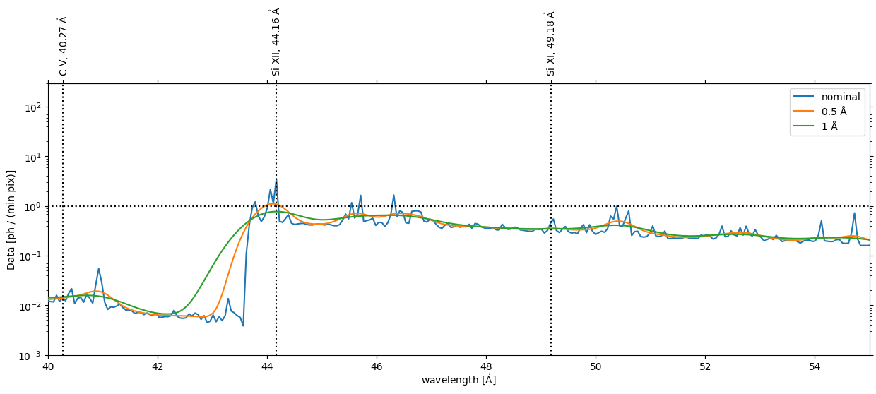
ax.set_xlim(ax.wcs.world_to_pixel([40,55]*u.angstrom))
ax.legend(loc=1)
WARNING: UnitsWarning: The unit 'Angstrom' has been deprecated in the VOUnit standard. Suggested: 0.1nm. [astropy.units.format.utils]
[21]:
<matplotlib.legend.Legend at 0x28bbf4d00>
Comparisons in Different Bandpasses#
Trying to reconcile what is happening in the CHIANTI IDL GUI and what I’m doing here…I want to make sure what I’m doing here is not wrong and I’m not missing an order of magnitude somewhere
In my investigation with the IDL ch_ss GUI, the plot below is fairly consistent with what is calculated there, for the flare.dem dataset.
[22]:
fig = plt.figure(figsize=(15,5))
ax = fig.add_subplot(projection=intensity_flare)
intensity_flare.plot(axes_units='Angstrom', axes=ax, lw=1)
ax.set_xlim(ax.wcs.world_to_pixel([1,70]*u.angstrom))
ax.set_yscale('log')
ax.set_ylim(1e14,1e17)
WARNING: No observer defined on WCS, SpectralCoord will be converted without any velocity frame change [astropy.wcs.wcsapi.fitswcs]
[22]:
(100000000000000.0, 1e+17)
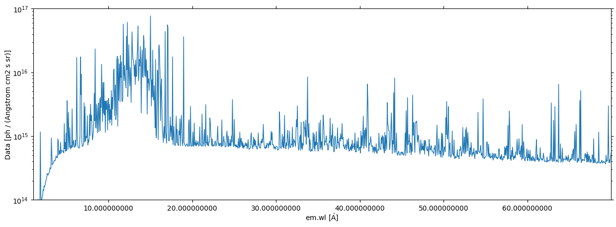
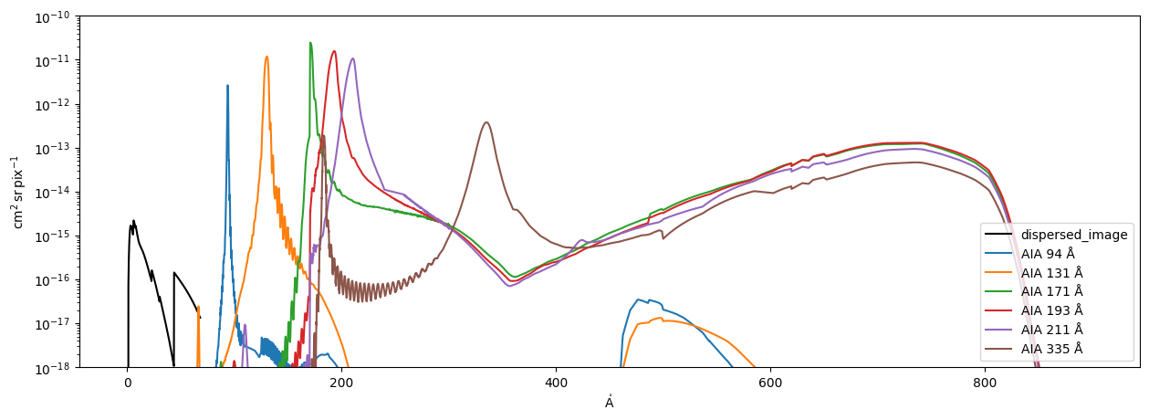
This seems really high, but then remembering we are multiplying by the following instrument response (in appropriate units)
[23]:
with quantity_support():
    plt.plot(chan.wavelength, chan.plate_scale * chan.effective_area * chan.spectral_resolution * 1 * u.pix)
plt.yscale('log')
/Users/wtbarnes/mambaforge/envs/mocksipipeline/lib/python3.9/site-packages/astropy/units/quantity.py:626: RuntimeWarning: divide by zero encountered in divide
  result = super().__array_ufunc__(function, method, *arrays, **kwargs)
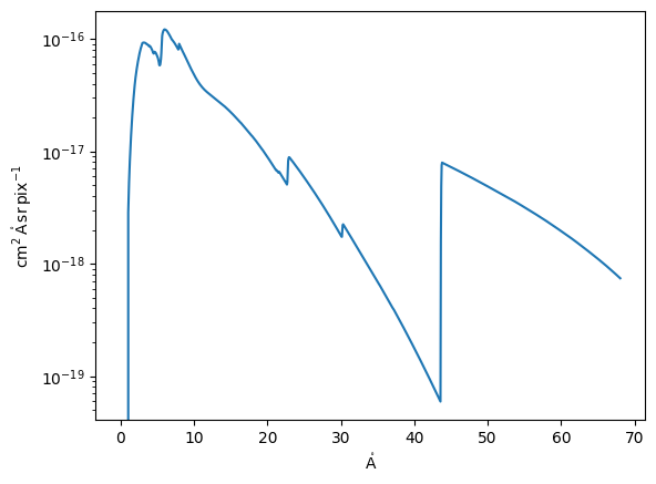
Just eyballing things, you can see that we’re only just barely getting above 1 ph pix\(^{-1}\) s\(^{-1}\) near 10 Å
So then a natural question is: if we were to observe this same “patch of Sun” with AIA, what would we see?
[24]:
class ChannelAIA(aiapy.response.Channel):

    @property
    @u.quantity_input
    def spectral_resolution(self):
        return np.diff(self.wavelength)[0] / u.pix
Let’s first compare all of the response functions in appropriate units
[25]:
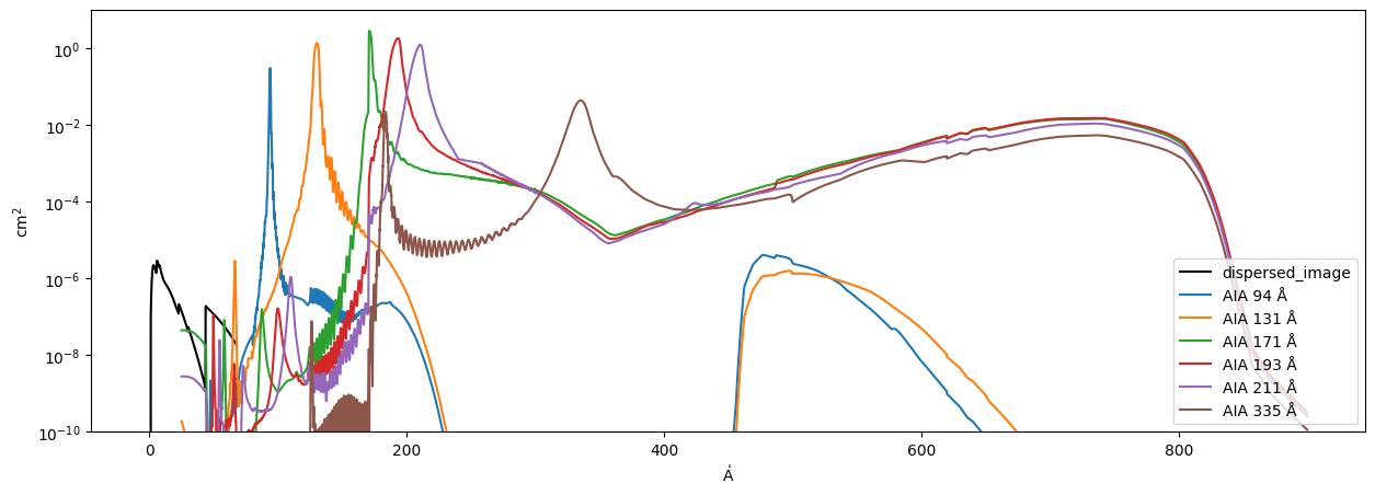
fig = plt.figure(figsize=(15,5))
ax = fig.add_subplot()
with quantity_support():
    ax.plot(chan.wavelength, chan.effective_area, label=chan.name, color='k')
    for aia_wave in [94, 131, 171, 193, 211, 335]*u.angstrom:
        chan_aia = ChannelAIA(aia_wave)
        ax.plot(chan_aia.wavelength, chan_aia.effective_area, label=f'AIA {chan_aia.name} Å')
ax.set_yscale('log')
ax.legend(loc=4)
ax.set_ylim(1e-10, 1e1)
[25]:
(1e-10, 10.0)
[26]:
fig = plt.figure(figsize=(15,5))
ax = fig.add_subplot()
with quantity_support():
    ax.plot(chan.wavelength, chan.plate_scale * chan.effective_area,
             label=chan.name, color='k')
    for aia_wave in [94, 131, 171, 193, 211, 335]*u.angstrom:
        chan_aia = ChannelAIA(aia_wave)
        ax.plot(chan_aia.wavelength, chan_aia.effective_area*chan_aia.plate_scale,
                label=f'AIA {chan_aia.name} Å')
ax.set_yscale('log')
ax.legend(loc=4)
ax.set_ylim(1e-18, 1e-10)
[26]:
(1e-18, 1e-10)
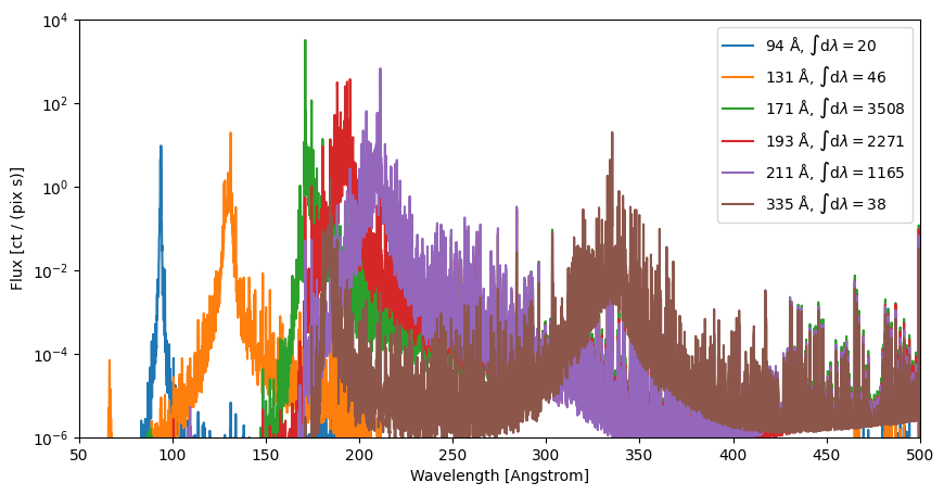
Let’s look first at the active region case. Looking below, we can see that we are getting pretty typical (based on AIA AR observations) numbers here. The numbers in the legend show what we’d expect to actually observe in an AIA pixel.
[27]:
fig = plt.figure(figsize=(10,5))
ax = fig.add_subplot()
for aia_wave in [94, 131, 171, 193, 211, 335]*u.angstrom:
    chan_aia = ChannelAIA(aia_wave)
    flux_ar_aia = convolve_with_response(intensity_ar, chan_aia, electrons=False, )
    flux_ar_aia = ndcube.NDCube(flux_ar_aia.data*flux_ar_aia.unit*chan_aia.gain,
                                wcs=flux_ar_aia.wcs)
    summed_counts = flux_ar_aia.data.sum()
    ax.plot(chan_aia.wavelength, flux_ar_aia.data, label=f'{aia_wave.value:.0f} Å, $\int\mathrm{{d}}\lambda={summed_counts:.0f}$')
ax.set_yscale('log')
ax.set_ylim(1e-6, 1e4)
ax.set_xlim(50, 500)
ax.set_ylabel(f'Flux [{flux_ar_aia.unit}]')
ax.set_xlabel(f'Wavelength [{chan_aia.wavelength.unit}]')
ax.legend(ncol=1)
[27]:
<matplotlib.legend.Legend at 0x28b821640>
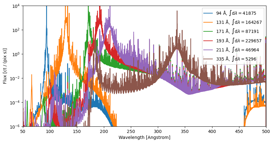
[28]:
fig = plt.figure(figsize=(10,5))
ax = fig.add_subplot()
for aia_wave in [94, 131, 171, 193, 211, 335]*u.angstrom:
    chan_aia = ChannelAIA(aia_wave)
    flux_flare_aia = convolve_with_response(intensity_flare, chan_aia, electrons=False, )
    flux_flare_aia = ndcube.NDCube(flux_flare_aia.data*flux_flare_aia.unit*chan_aia.gain,
                                wcs=flux_flare_aia.wcs)
    summed_counts = flux_flare_aia.data.sum()
    ax.plot(chan_aia.wavelength, flux_flare_aia.data, label=f'{aia_wave.value:.0f} Å, $\int\mathrm{{d}}\lambda={summed_counts:.0f}$')
ax.set_yscale('log')
ax.set_ylim(1e-6, 1e4)
ax.set_xlim(50, 500)
ax.set_ylabel(f'Flux [{flux_flare_aia.unit}]')
ax.set_xlabel(f'Wavelength [{chan_aia.wavelength.unit}]')
ax.legend(ncol=1)
[28]:
<matplotlib.legend.Legend at 0x28b9d3520>
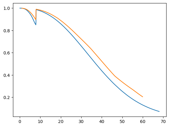
[35]:
plt.plot(chan.wavelength, chan.filter_transmission)
plt.plot(chan._wavelength_data, chan._data['filter'])
#plt.yscale('log')
[35]:
[<matplotlib.lines.Line2D at 0x28b77fc70>]
[ ]: