Flare Line Diagnostics#
Here, we assess the SNR in a number of flare lines for classes M1 and above
[1]:
import asdf
from astropy.coordinates import SkyCoord
import astropy.table
import astropy.units as u
from astropy.visualization import quantity_support
from astropy.wcs.utils import wcs_to_celestial_frame
import fiasco
import matplotlib.pyplot as plt
import ndcube
import numpy as np
from scipy.interpolate import interp1d
from sunpy.coordinates import get_earth

from mocksipipeline.modeling import convolve_with_response, _blur_spectra
from mocksipipeline.instrument.configuration import moxsi_slot_spectrogram_pinhole, moxsi_slot
[2]:
def annotate_lines(axis, line_list, flux, color, unit=None, rtol=0.1):
    wavelength = flux.axis_world_coords(0)[0]
    data = flux.to(flux.unit if unit is None else unit).data
    for row in line_list:
        i_x = flux.wcs.world_to_array_index(u.Quantity([row['wavelength']]))
        if data[i_x] / data.max() < rtol:
            continue
        axis.annotate(
            f'{row["ion name"]}, {row["wavelength"].to_string(format="latex_inline", precision=5)}',
            (wavelength[i_x].to_value(), data[i_x]),
            xytext=(0, 150),
            textcoords='offset points',
            rotation=90,
            color=color,
            horizontalalignment='center',
            verticalalignment='center',
            arrowprops=dict(color=color, arrowstyle='-', ls='--'),
        )
Creating a flare line list#
Load the line list and estimate the MOXSI flux from the CHIANTI intensities
[4]:
channel_o1 = moxsi_slot_spectrogram_pinhole.channel_list[12]
[5]:
channel_o1
[5]:
MOXSI Detector Channel--spectrogram_pinhole
-----------------------------------
Spectral order: 1
Filter: Al+Al2O3, 150.000 nm
Detector dimensions: (1504, 2000)
Wavelength range: [0.0 Angstrom, 83.61862217082933 Angstrom]
Spectral plate scale: 0.07179487179487179 Angstrom / pix
Spatial plate scale: [7.40437766 7.40437766] arcsec / pix
Reference pixel: [1000.  752.    0.] pix
aperture: Circular Aperture
-------------------------
diameter: 44.0 micron
area: 1.5205308443374597e-05 cm2
[6]:
earth_obs = get_earth('2020-01-01')
hpc_frame = wcs_to_celestial_frame(channel_o1.get_wcs(earth_obs))
source_loc = SkyCoord(Tx=0*u.arcsec, Ty=0*u.arcsec, frame=hpc_frame)
WARNING: FITSFixedWarning: 'datfix' made the change 'Set MJD-OBS to 58849.000000 from DATE-OBS'. [astropy.wcs.wcs]
WARNING: FITSFixedWarning: 'unitfix' made the change 'Changed units:
  'angstrom' -> 'Angstrom'. [astropy.wcs.wcs]
First, load the line list and convert intensities to units of the MOXSI detector. Note that we can carry out a similar process for the AR case using the AR intensity and the lower energy flare classes.
[7]:
full_line_list = astropy.table.QTable.read('../data/line_lists/full-line-list.asdf')
full_line_list = full_line_list[['ion name',
                                 'wavelength',
                                 'max temperature_flare_ext',
                                 'intensity (coronal)_flare_ext',
                                 'intensity (coronal)_active_region']]
full_line_list['energy'] = full_line_list['wavelength'].to('keV', equivalencies=u.spectral())
# Convert intensities to instrument units
f_ea_interp = interp1d(channel_o1.wavelength.to_value('AA'), channel_o1.effective_area.to_value('cm2'),)
ea_interp = f_ea_interp(full_line_list['wavelength'].to_value('AA')) * u.cm**2
full_line_list['intensity (coronal)_flare_ext'] = (full_line_list['intensity (coronal)_flare_ext'] *
                                                   ea_interp * channel_o1.pixel_solid_angle)
full_line_list.rename_column('intensity (coronal)_flare_ext', r'flare\_ext')
full_line_list['intensity (coronal)_active_region'] = (full_line_list['intensity (coronal)_active_region'] *
                                                       ea_interp * channel_o1.pixel_solid_angle).to('ph/pix/h')
full_line_list.rename_column('intensity (coronal)_active_region', r'active\_region')
# Add approximate formation temperature
temperature_grid = 10**np.arange(5.5,7.5,0.05)*u.K
all_chianti_ions = [fiasco.Ion(i, temperature_grid) for i in fiasco.list_ions(fiasco.defaults['hdf5_dbase_root'])]
ioneq_tmax = {i.ion_name_roman: i.formation_temperature for i in all_chianti_ions}
full_line_list['$T_{max}$'] = list(map(lambda x: ioneq_tmax[x].to('MK'), full_line_list['ion name']))
# Add FIP information
all_chianti_elements = [fiasco.Element(el, 1*u.MK) for el in fiasco.list_elements(fiasco.defaults['hdf5_dbase_root'])]
element_fip = {el.atomic_symbol: el[0].ip for el in all_chianti_elements}
full_line_list['IP'] = list(map(lambda x: element_fip[x.split()[0]].to('eV'), full_line_list['ion name']))
full_line_list['FIP'] = list(map(lambda x: 'low' if x<=10*u.eV else 'high', full_line_list['IP']))
# Add information about which moxsi pixel corresponds to which wavelength
full_line_list['MOXSI pixel'] = channel_o1.get_wcs(earth_obs).world_to_array_index(source_loc, full_line_list['wavelength'])[-1]
# Reorder columns
full_line_list = full_line_list[[
    'ion name',
    'wavelength',
    'energy',
    'MOXSI pixel',
    '$T_{max}$',
    'IP',
    'FIP',
    r'flare\_ext',
]]
full_line_list.sort(keys='wavelength')
WARNING: UnitsWarning: The unit 'Angstrom' has been deprecated in the VOUnit standard. Suggested: 0.1nm. [astropy.units.format.utils]
/Users/wtbarnes/mambaforge/envs/mocksipipeline-dev/lib/python3.11/site-packages/astropy/units/equivalencies.py:141: RuntimeWarning: divide by zero encountered in divide
  (si.m, si.J, lambda x: hc / x),
/Users/wtbarnes/mambaforge/envs/mocksipipeline-dev/lib/python3.11/site-packages/xrt/backends/raycing/materials.py:253: UserWarning: Reading `.npy` or `.npz` file required additional header parsing as it was created on Python 2. Save the file again to speed up loading and avoid this warning.
  ef1f2 = (np.array(res[self.name+'_E']),
/Users/wtbarnes/mambaforge/envs/mocksipipeline-dev/lib/python3.11/site-packages/xrt/backends/raycing/materials.py:254: UserWarning: Reading `.npy` or `.npz` file required additional header parsing as it was created on Python 2. Save the file again to speed up loading and avoid this warning.
  np.array(res[self.name+'_f1']),
/Users/wtbarnes/mambaforge/envs/mocksipipeline-dev/lib/python3.11/site-packages/xrt/backends/raycing/materials.py:255: UserWarning: Reading `.npy` or `.npz` file required additional header parsing as it was created on Python 2. Save the file again to speed up loading and avoid this warning.
  np.array(res[self.name+f2key]))
/Users/wtbarnes/mambaforge/envs/mocksipipeline-dev/lib/python3.11/site-packages/astropy/units/equivalencies.py:141: RuntimeWarning: divide by zero encountered in divide
  (si.m, si.J, lambda x: hc / x),
WARNING: UnitsWarning: 'ph/pix/h' contains multiple slashes, which is discouraged by the FITS standard [astropy.units.format.generic]
WARNING: FITSFixedWarning: 'datfix' made the change 'Set MJD-OBS to 58849.000000 from DATE-OBS'. [astropy.wcs.wcs]
WARNING: FITSFixedWarning: 'unitfix' made the change 'Changed units:
  'angstrom' -> 'Angstrom'. [astropy.wcs.wcs]
WARNING: No observer defined on WCS, SpectralCoord will be converted without any velocity frame change [astropy.wcs.wcsapi.fitswcs]
We want to avoid cases where we include lines that are actually weak, but get grouped into the same pixel as strong lines and thus appear as if they’re just as strong. Thus, we’ll group by MOXSI pixel and if a particular line is significantly below that line in that pixel, then we drop that line
[9]:
max_threshold = 0.05
group_tables = []
for group in full_line_list.group_by('MOXSI pixel').groups:
    group_tables.append(group[group['flare\\_ext'] >= group['flare\\_ext'].max() * max_threshold])
full_line_list = astropy.table.vstack(group_tables)
Then, load the reference flare spectra
[10]:
goes_class = ['m1', 'm5', 'x5']
flare_spectra = []
with asdf.open('../data/reference_spectra/caspi_flare_spectra.asdf', copy_arrays=True) as af:
    for gc in goes_class:
        flare_spectra.append((gc, ndcube.NDCube(af.tree[gc]['data'], wcs=af.tree[gc]['wcs'])))
flare_spectra = ndcube.NDCollection(flare_spectra, aligned_axes=(0,))
WARNING: UnitsWarning: The unit 'Angstrom' has been deprecated in the VOUnit standard. Suggested: 0.1nm. [astropy.units.format.utils]
Now, compute the MOXSI counts for a source location at disk center as a function of pixel
First, let’s just look at the flux in each line in first order
[11]:
flux_columns = {}
for gc in goes_class:
    flux = convolve_with_response(flare_spectra[gc], channel_o1, include_gain=False)
    #flux = _blur_spectra(flux, blur / channel_o1.spatial_plate_scale[0] * channel_o1.spectral_plate_scale, channel_o1)
    #indices = flux.wcs.world_to_array_index(full_line_list['wavelength'])
    # NOTE: Calling w2ai on an array when the WCS is 1D reverses the order of the returned indices (!!!)
    #indices = np.array(indices)[::-1]
    f_interp = interp1d(flux.axis_world_coords(0)[0].to_value('AA'), flux.data, kind='nearest')
    flux_columns[gc.capitalize()] = (f_interp(full_line_list['wavelength'].to_value('AA'))*flux.unit).to('ph/pix/s')
flare_snr_table = astropy.table.QTable(flux_columns)
flare_snr_table = astropy.table.hstack([full_line_list,flare_snr_table])
flare_snr_table.sort(keys='wavelength')
/Users/wtbarnes/mambaforge/envs/mocksipipeline-dev/lib/python3.11/site-packages/astropy/units/equivalencies.py:141: RuntimeWarning: divide by zero encountered in divide
  (si.m, si.J, lambda x: hc / x),
/Users/wtbarnes/mambaforge/envs/mocksipipeline-dev/lib/python3.11/site-packages/xrt/backends/raycing/materials.py:253: UserWarning: Reading `.npy` or `.npz` file required additional header parsing as it was created on Python 2. Save the file again to speed up loading and avoid this warning.
  ef1f2 = (np.array(res[self.name+'_E']),
/Users/wtbarnes/mambaforge/envs/mocksipipeline-dev/lib/python3.11/site-packages/xrt/backends/raycing/materials.py:254: UserWarning: Reading `.npy` or `.npz` file required additional header parsing as it was created on Python 2. Save the file again to speed up loading and avoid this warning.
  np.array(res[self.name+'_f1']),
/Users/wtbarnes/mambaforge/envs/mocksipipeline-dev/lib/python3.11/site-packages/xrt/backends/raycing/materials.py:255: UserWarning: Reading `.npy` or `.npz` file required additional header parsing as it was created on Python 2. Save the file again to speed up loading and avoid this warning.
  np.array(res[self.name+f2key]))
WARNING: UnitsWarning: 'ph/pix/s' contains multiple slashes, which is discouraged by the FITS standard [astropy.units.format.generic]
The next thing we need to do is make a cut in SNR to eliminate those lines we don’t have a chance of seeing. We require that this threshold be met at the M1 level and above
[12]:
threshold = 0.1 * u.photon / u.pix / u.s
[13]:
flare_snr_table = flare_snr_table[flare_snr_table['M1'] > threshold]
Finally, now that we’ve really pared down the table, let’s compute a \(T_{max}\) based on the contribution function
[14]:
contribution_functions = {}
for ion_name in np.unique(flare_snr_table['ion name']):
    ion = fiasco.Ion(ion_name, temperature_grid)
    #density = 1e15*u.K/(u.cm**3)/ion.temperature
    density = 1e10 * u.cm**(-3)
    goft = ion.contribution_function(density, couple_density_to_temperature=False)
    transitions = ion.transitions.wavelength[~ion.transitions.is_twophoton]
    contribution_functions[ion_name] = (transitions, goft)
goft_col = []
for row in flare_snr_table:
    _t, _g = contribution_functions[row['ion name']]
    idx = np.argmin(np.abs(_t - row['wavelength']))
    goft_col.append(_g[:,0,idx])
flare_snr_table['$T_{max,G}$'] = list(map(lambda x: temperature_grid[np.argmax(x)].to('MK'), goft_col))
WARNING: No proton data available for Al 12. Not including proton excitation and de-excitation in level populations calculation. [fiasco.ions]
WARNING: No proton data available for Ar 9. Not including proton excitation and de-excitation in level populations calculation. [fiasco.ions]
WARNING: No proton data available for Fe 16. Not including proton excitation and de-excitation in level populations calculation. [fiasco.ions]
WARNING: No proton data available for Fe 17. Not including proton excitation and de-excitation in level populations calculation. [fiasco.ions]
WARNING: No proton data available for Fe 24. Not including proton excitation and de-excitation in level populations calculation. [fiasco.ions]
WARNING: No proton data available for Mg 10. Not including proton excitation and de-excitation in level populations calculation. [fiasco.ions]
WARNING: No proton data available for Mg 11. Not including proton excitation and de-excitation in level populations calculation. [fiasco.ions]
WARNING: No proton data available for Mg 12. Not including proton excitation and de-excitation in level populations calculation. [fiasco.ions]
WARNING: No proton data available for N 7. Not including proton excitation and de-excitation in level populations calculation. [fiasco.ions]
WARNING: No proton data available for Ne 9. Not including proton excitation and de-excitation in level populations calculation. [fiasco.ions]
WARNING: No proton data available for Ne 10. Not including proton excitation and de-excitation in level populations calculation. [fiasco.ions]
WARNING: No proton data available for Ni 19. Not including proton excitation and de-excitation in level populations calculation. [fiasco.ions]
WARNING: No proton data available for O 7. Not including proton excitation and de-excitation in level populations calculation. [fiasco.ions]
WARNING: No proton data available for O 8. Not including proton excitation and de-excitation in level populations calculation. [fiasco.ions]
WARNING: No proton data available for Si 12. Not including proton excitation and de-excitation in level populations calculation. [fiasco.ions]
WARNING: No proton data available for Si 13. Not including proton excitation and de-excitation in level populations calculation. [fiasco.ions]
WARNING: No proton data available for Si 14. Not including proton excitation and de-excitation in level populations calculation. [fiasco.ions]
One last reordering of the columns
[15]:
flare_snr_table = flare_snr_table[[
    'ion name',
    'wavelength',
    'energy',
    'MOXSI pixel',
    '$T_{max}$',
    '$T_{max,G}$',
    'IP',
    'FIP',
    r'flare\_ext',
    'M1',
    'M5',
    'X5',
]]
flare_snr_table.sort(keys='wavelength')
[18]:
flare_snr_table
[18]:
| ion name | wavelength | energy | MOXSI pixel | $T_{max}$ | $T_{max,G}$ | IP | FIP | flare\_ext | M1 | M5 | X5 |
|---|---|---|---|---|---|---|---|---|---|---|---|
| Angstrom | keV | MK | MK | eV | ph / (pix s) | ph / (pix s) | ph / (pix s) | ph / (pix s) | |||
| str9 | float64 | float64 | int64 | float64 | float64 | float64 | str4 | float64 | float64 | float64 | float64 |
| Si XIV | 6.1803998947143555 | 2.0060869934845944 | 1086 | 12.589254117941508 | 15.848931924610914 | 8.151683322378426 | low | 2.77150168778808 | 0.19092068163432263 | 0.7726231879135387 | 5.958959528393517 |
| Si XIV | 6.185800075531006 | 2.0043356868845636 | 1086 | 12.589254117941508 | 15.848931924610914 | 8.151683322378426 | low | 1.3860111467366312 | 0.19092068163432263 | 0.7726231879135387 | 5.958959528393517 |
| Si XIII | 6.647900104522705 | 1.8650129587364168 | 1093 | 4.466835921509589 | 9.999999999999877 | 8.151683322378426 | low | 2.5822871994428858 | 0.3885113286497903 | 1.698976270422117 | 16.01591653315726 |
| Si XIII | 6.688199996948242 | 1.853775283181917 | 1093 | 4.466835921509589 | 8.91250938133735 | 8.151683322378426 | low | 0.3761381491317149 | 0.10098502280776257 | 0.44102727439977624 | 4.266389879196875 |
| Mg XII | 7.105800151824951 | 1.7448309238102893 | 1099 | 7.943282347242723 | 9.999999999999877 | 7.646231981257862 | low | 0.17467006358746945 | 0.1656320158333378 | 0.7183016932647145 | 6.601093936462812 |
| Mg XII | 7.106900215148926 | 1.7445608448099217 | 1099 | 7.943282347242723 | 9.999999999999877 | 7.646231981257862 | low | 0.08751833495453741 | 0.1656320158333378 | 0.7183016932647145 | 6.601093936462812 |
| Al XII | 7.757299900054932 | 1.5982906427573111 | 1108 | 3.548133892335724 | 7.943282347242723 | 5.985755006111463 | low | 0.08337538277386186 | 0.18914877351453044 | 0.809461063592222 | 7.7635870033849725 |
| Mg XI | 9.231200218200684 | 1.3430994399704055 | 1129 | 2.818382931264432 | 6.309573444801865 | 7.646231981257862 | low | 0.0927484731152775 | 0.32627721731984916 | 1.380182779037875 | 13.309287922783925 |
| Fe XXII | 9.240699768066406 | 1.3417187176847714 | 1129 | 12.589254117941508 | 14.125375446227352 | 7.902380855536887 | low | 0.05437801101715639 | 0.32627721731984916 | 1.380182779037875 | 13.309287922783925 |
| Fe XXI | 9.475000381469727 | 1.3085403001743023 | 1132 | 11.220184543019492 | 12.589254117941508 | 7.902380855536887 | low | 0.3768521339716754 | 0.15039044472368926 | 0.379728592767079 | 2.514803350288388 |
| Fe XIX | 9.690500259399414 | 1.2794406389178963 | 1135 | 8.91250938133735 | 9.999999999999877 | 7.902380855536887 | low | 0.04869614714994042 | 0.11205044615089021 | 0.46672916307593104 | 4.468277244525059 |
| Ni XXV | 9.967000007629395 | 1.2439470085110327 | 1139 | 19.9526231496885 | 19.9526231496885 | 7.637426623485137 | low | 0.08248935516333857 | 0.1311527241012997 | 0.5724325735074639 | 5.512369204832659 |
| Fe XXI | 9.972999572753906 | 1.24319867386662 | 1139 | 11.220184543019492 | 12.589254117941508 | 7.902380855536887 | low | 0.04903446378849213 | 0.1311527241012997 | 0.5724325735074639 | 5.512369204832659 |
| Ni XIX | 9.977100372314453 | 1.2426876928816424 | 1139 | 5.623413251903433 | 7.943282347242723 | 7.637426623485137 | low | 0.041458107113121485 | 0.1311527241012997 | 0.5724325735074639 | 5.512369204832659 |
| Ne X | 10.238499641418457 | 1.2109606170384482 | 1143 | 4.466835921509589 | 6.309573444801865 | 21.564534438226993 | high | 0.06612673171119207 | 0.1079215555330552 | 0.45379970093992866 | 4.336895828035151 |
| Fe XVII | 10.503999710083008 | 1.180352264425381 | 1146 | 3.9810717055349367 | 6.309573444801865 | 7.902380855536887 | low | 0.05176327154590408 | 0.15128073555557275 | 0.6907915103592993 | 6.8035718533056615 |
| ... | ... | ... | ... | ... | ... | ... | ... | ... | ... | ... | ... |
| O VII | 21.803600311279297 | 0.5686409430696706 | 1304 | 0.8912509381337421 | 1.9952623149688664 | 13.61805488299139 | high | 0.0015388947425488844 | 0.20736578083325655 | 0.22033572481976407 | 0.3664870391017608 |
| O VII | 22.097700119018555 | 0.5610728617250639 | 1308 | 0.8912509381337421 | 1.9952623149688664 | 13.61805488299139 | high | 0.006140919497209702 | 0.3253953174442503 | 0.3516523446072838 | 0.64856053729616 |
| N VII | 24.779199600219727 | 0.5003559454442621 | 1345 | 1.5848931924611043 | 1.9952623149688664 | 14.534097255011275 | high | 0.013948315680010676 | 0.1468899377200163 | 0.19791373132046583 | 0.7718378776017261 |
| N VII | 24.78459930419922 | 0.5002469352498016 | 1345 | 1.5848931924611043 | 1.9952623149688664 | 14.534097255011275 | high | 0.006960987099128203 | 0.1468899377200163 | 0.19791373132046583 | 0.7718378776017261 |
| Si XI | 43.762001037597656 | 0.2833147376571756 | 1610 | 1.5848931924611043 | 1.7782794100389119 | 8.151683322378426 | low | 0.003514375584198909 | 0.10407851722097457 | 0.1379839653546789 | 0.5217646851356907 |
| Si XII | 44.01860046386719 | 0.2816631994808037 | 1613 | 1.9952623149688664 | 2.238721138568324 | 8.151683322378426 | low | 0.031324790904888475 | 0.1437587333670237 | 0.27632399502797744 | 1.7775620686470603 |
| Mg X | 44.04999923706055 | 0.28146243037590957 | 1614 | 1.1220184543019585 | 1.2589254117941608 | 7.646231981257862 | low | 0.001538411874001072 | 0.10138900285630766 | 0.1946142488219808 | 1.2502676590741986 |
| Mg X | 44.04999923706055 | 0.28146243037590957 | 1614 | 1.1220184543019585 | 1.2589254117941608 | 7.646231981257862 | low | 0.0023253067918382305 | 0.10138900285630766 | 0.1946142488219808 | 1.2502676590741986 |
| Si XII | 44.160301208496094 | 0.2807594038995066 | 1615 | 1.9952623149688664 | 2.238721138568324 | 8.151683322378426 | low | 0.056478242720285794 | 0.3459607905543416 | 0.6514403554257849 | 4.1115770161745875 |
| Si XII | 45.69060134887695 | 0.27135602240491785 | 1636 | 1.9952623149688664 | 2.238721138568324 | 8.151683322378426 | low | 0.025387291189323067 | 0.14828969378704013 | 0.27329797601918404 | 1.6889536403974332 |
| Si XI | 49.17599868774414 | 0.25212339706707393 | 1685 | 1.5848931924611043 | 1.7782794100389119 | 8.151683322378426 | low | 0.00019421343022137528 | 0.11622844011369246 | 0.1396861387703588 | 0.40526176497891203 |
| Ar IX | 49.18550109863281 | 0.25207468799509003 | 1685 | 0.7079457843841358 | 1.1220184543019585 | 15.759606666004402 | high | 6.688484348572473e-05 | 0.11622844011369246 | 0.1396861387703588 | 0.40526176497891203 |
| Fe XVI | 50.361000061035156 | 0.24619089828029078 | 1701 | 2.818382931264432 | 2.818382931264432 | 7.902380855536887 | low | 0.012327115945859805 | 0.13784541053797664 | 0.28445874538050137 | 1.9476444322558906 |
| Fe XVI | 54.709999084472656 | 0.22662072840061226 | 1762 | 2.818382931264432 | 2.818382931264432 | 7.902380855536887 | low | 0.011105113970655162 | 0.10541894645425448 | 0.19299346912618265 | 1.1863695616483072 |
| Fe XVI | 63.71099853515625 | 0.19460407352552284 | 1887 | 2.818382931264432 | 2.818382931264432 | 7.902380855536887 | low | 0.00859276898298539 | 0.10946116201978805 | 0.18853736368045634 | 1.0857416459736378 |
| Si VIII | 63.731998443603516 | 0.19453995082692085 | 1888 | 0.8912509381337421 | 0.9999999999999959 | 8.151683322378426 | low | 1.8936964471402224e-05 | 0.10946116201978805 | 0.18853736368045634 | 1.0857416459736378 |
Now, save the line table
[19]:
flare_snr_table.write('../data/line_lists/flare-line-table.asdf')
WARNING: UnitsWarning: The unit 'Angstrom' has been deprecated in the VOUnit standard. Suggested: 0.1nm. [astropy.units.format.utils]
WARNING: UnitsWarning: The unit 'Angstrom' has been deprecated in the VOUnit standard. Suggested: 0.1nm. [astropy.units.format.utils]
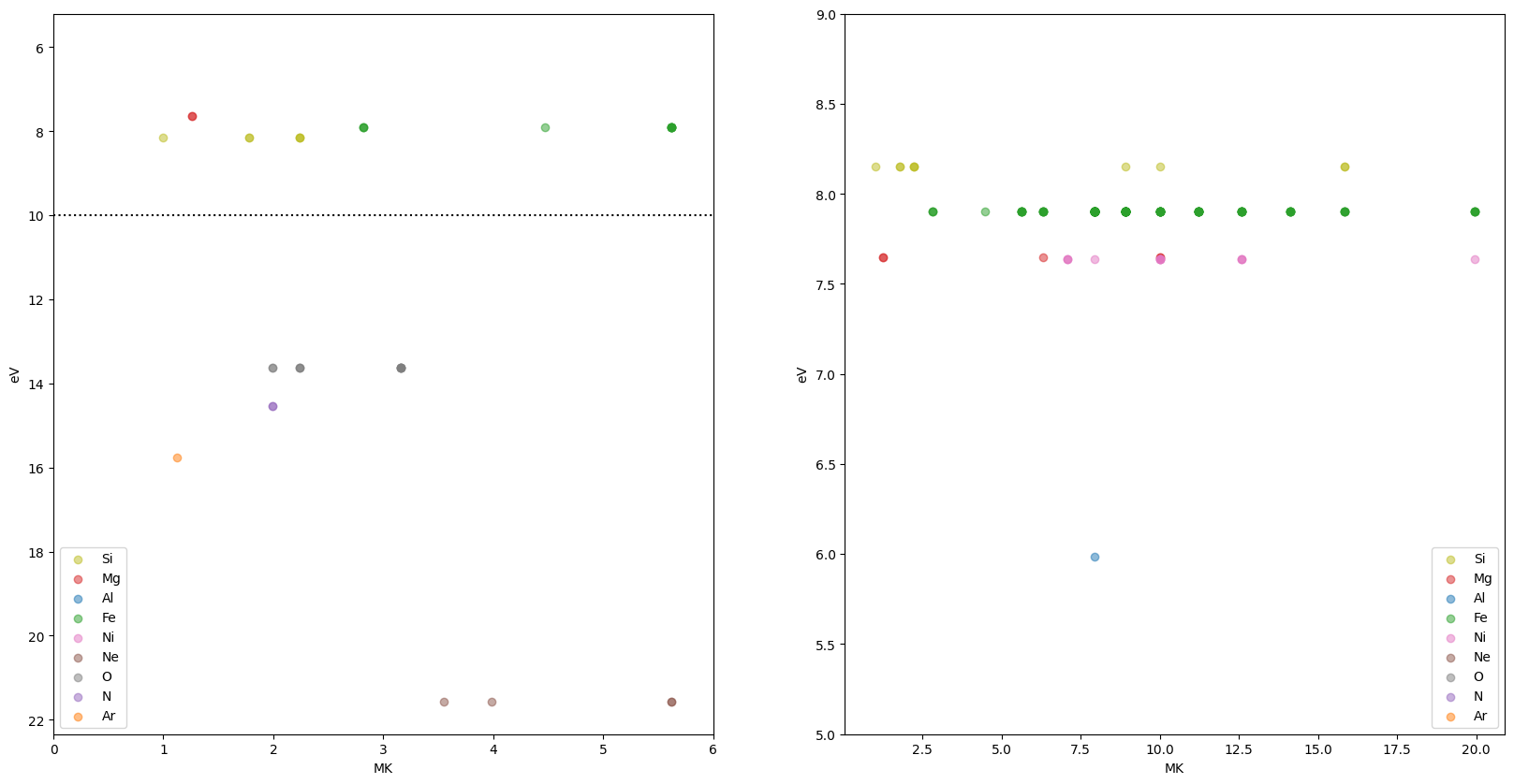
Assessing Relationship between formation temperature and IP#
Plot ionization potential versus formation temperature
[15]:
el_colors = {el: f'C{i}' for i,el in enumerate(np.unique(list(map(lambda x: x.split()[0], flare_snr_table['ion name']))))}
with quantity_support():
    fig = plt.figure(figsize=(20,10))
    # Contribution function
    ax = fig.add_subplot(121)
    for row in flare_snr_table:
        ax.scatter(row['$T_{max,G}$'], row['IP'],
                   marker='.',
                   s=500,
                   color=el_colors[row['ion name'].split()[0]],
                   #s=row['X5']*1e3,
                   #alpha=0.25,
                   label=row['ion name'].split()[0])
    ax.axhline(y=10*u.eV, color='k', ls=':')
    ax.invert_yaxis()
    handles, labels = ax.get_legend_handles_labels()
    by_label = dict(zip(labels, handles))
    ax.legend(by_label.values(), by_label.keys(),loc=4)
    # Ionization fraction
    ax = fig.add_subplot(122,sharex=ax,sharey=ax)
    for row in flare_snr_table:
        ax.scatter(row['$T_{max}$'], row['IP'],
                   marker='.',
                   s=500,
                   color=el_colors[row['ion name'].split()[0]],
                   #s=row['X5']*1e3,
                   #alpha=0.25,
                   label=row['ion name'].split()[0])
    ax.axhline(y=10*u.eV, color='k', ls=':')

[16]:
with quantity_support():
    fig = plt.figure(figsize=(20,10))
    # Compare high and low FIP
    ax = fig.add_subplot(121)
    for row in flare_snr_table:
        ax.scatter(row['$T_{max,G}$'], row['IP'],
                   marker='o',
                   color=el_colors[row['ion name'].split()[0]],
                   #s=row['M5']*1e3,
                   alpha=0.5,
                   label=row['ion name'].split()[0])
    ax.axhline(y=10*u.eV, color='k', ls=':')
    handles, labels = ax.get_legend_handles_labels()
    by_label = dict(zip(labels, handles))
    ax.legend(by_label.values(), by_label.keys(), loc=3)
    ax.set_xlim(0,6)
    ax.invert_yaxis()
    # Compare temperature coverage
    ax = fig.add_subplot(122)
    for row in flare_snr_table:
        ax.scatter(row['$T_{max,G}$'], row['IP'],
                   marker='o',
                   color=el_colors[row['ion name'].split()[0]],
                   #s=row['M5']*1e3,
                   alpha=0.5,
                   label=row['ion name'].split()[0])
    ax.axhline(y=10*u.eV, color='k', ls=':')
    handles, labels = ax.get_legend_handles_labels()
    by_label = dict(zip(labels, handles))
    ax.legend(by_label.values(), by_label.keys(), loc=4)
    ax.set_ylim(5,9)
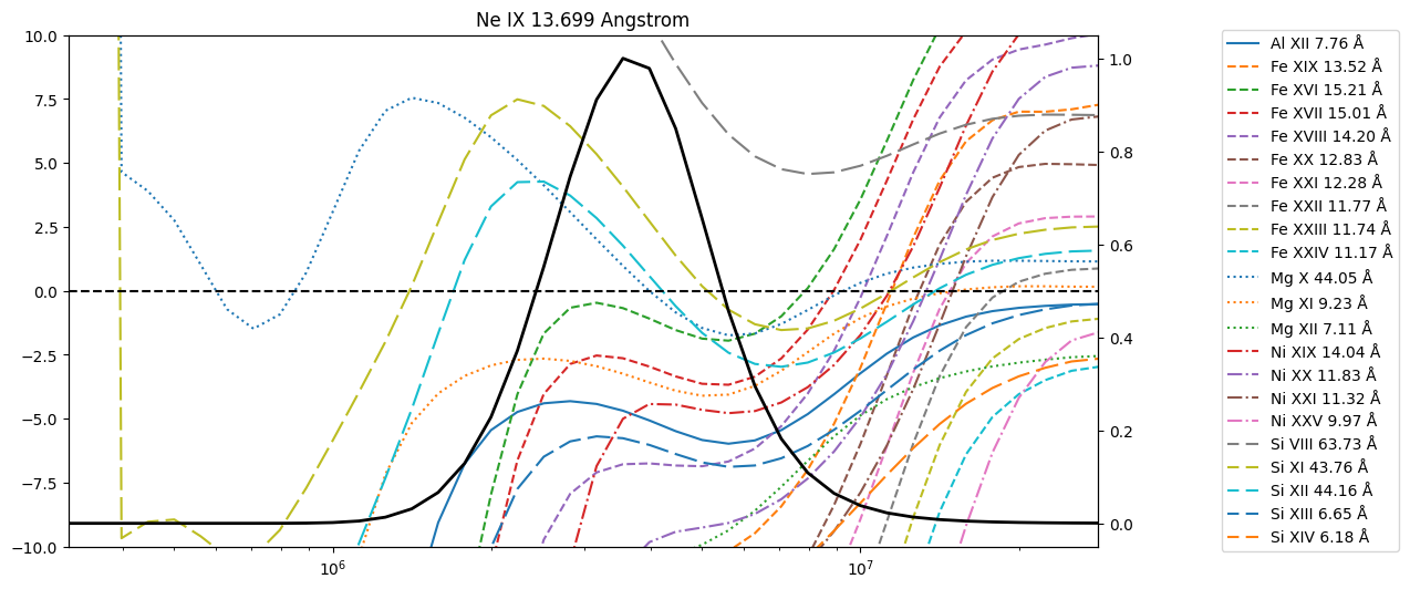
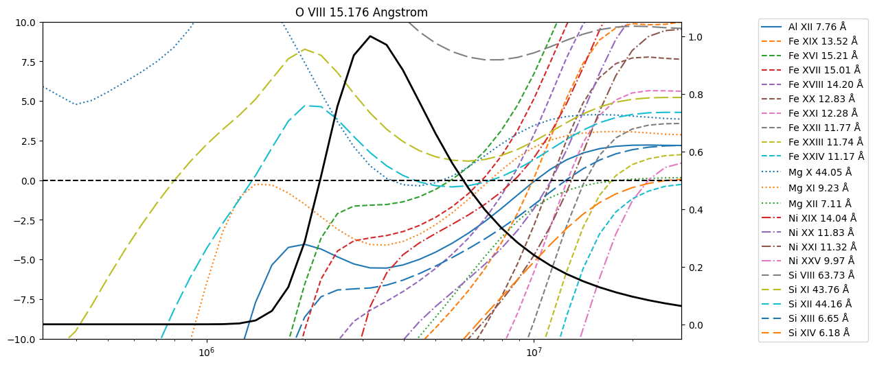
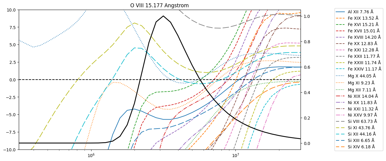
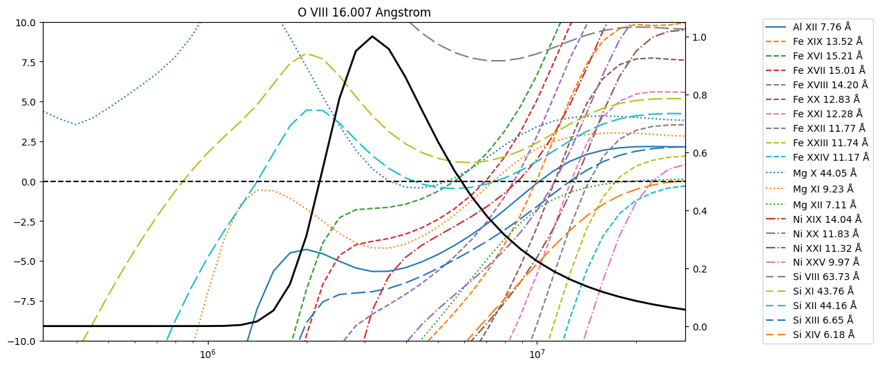
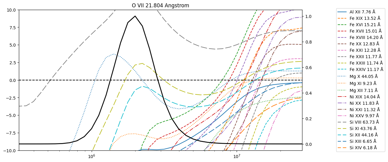
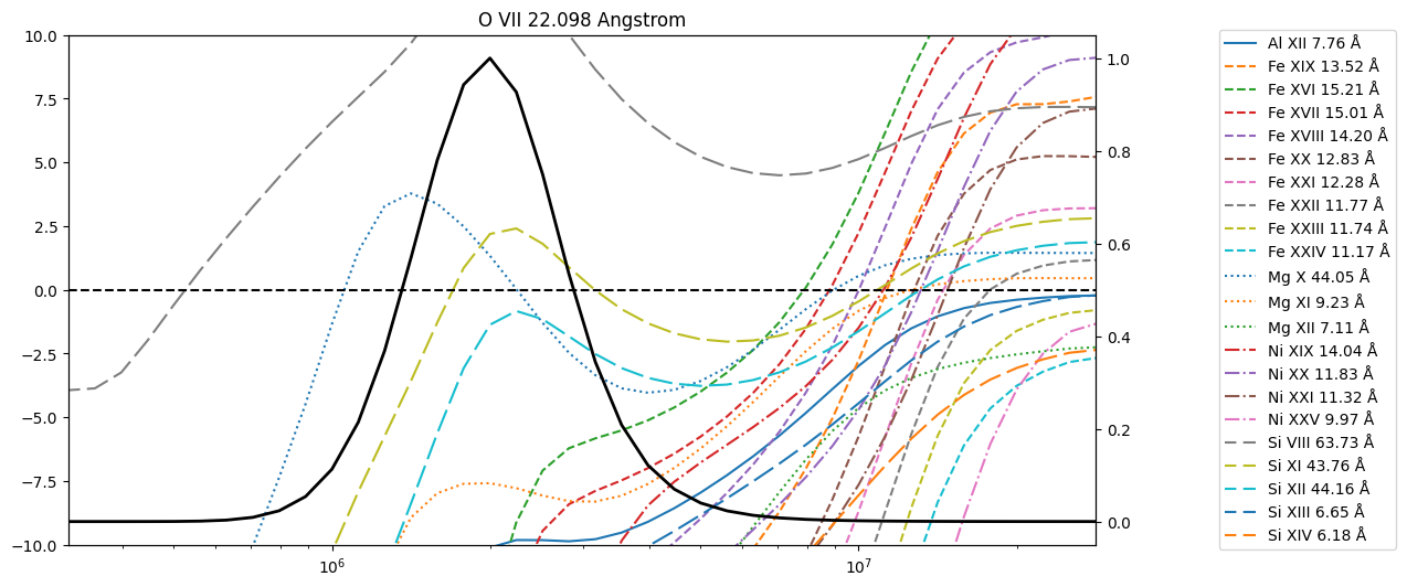
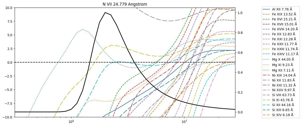
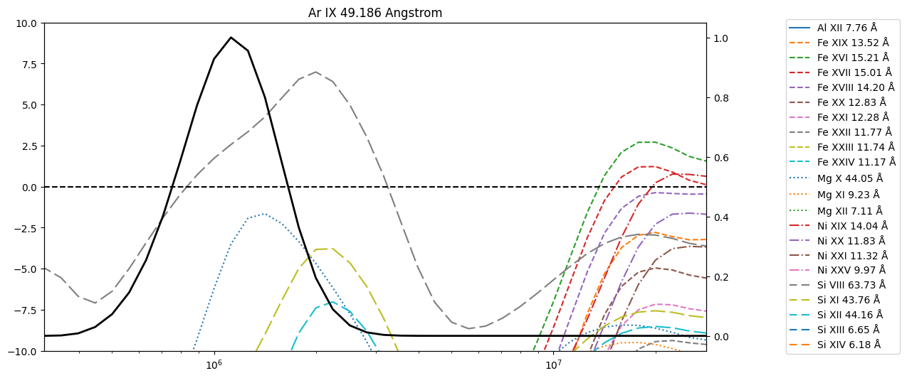
Assessing \(G(T)\) ratio for High and Low FIP Pairs#
[17]:
fig = plt.figure(figsize=(10,7))
ax = fig.add_subplot()
for goft,ion_name,fip in zip(goft_col, flare_snr_table['ion name'], flare_snr_table['FIP']):
    ax.plot(temperature_grid, goft, color=el_colors[ion_name.split()[0]], alpha=0.2 if fip=='low' else 1.0, label=ion_name.split()[0])
ax.set_xscale('log')
ax.set_yscale('log')
ax.set_ylim(1e-30, 1e-23)
ax.set_xlim(4e5, 2e7)
handles, labels = ax.get_legend_handles_labels()
by_label = dict(zip(labels, handles))
ax.legend(by_label.values(), by_label.keys())
[17]:
<matplotlib.legend.Legend at 0x1771e1510>

Maybe take ratios between the contribution functions of the high-FIP elements? Which ones are the most flat across the relevant temperature ranges?
[18]:
modded_table = flare_snr_table.copy()
modded_table['contribution function'] = goft_col
[19]:
low_fip_lines = modded_table[modded_table['FIP']=='low']
high_fip_lines = modded_table[modded_table['FIP']=='high']
[20]:
from cycler import cycler
ls_cycler = cycler(linestyle=['-', '--', ':', '-.', (5, (10, 3))])
el_linestyles = {el: ls for el,ls in zip(np.unique(list(map(lambda x: x.split()[0], low_fip_lines['ion name']))), ls_cycler)}
[22]:
for hf_row in high_fip_lines:#.group_by('ion name').groups:
    #hf_row = tab[np.argsort(tab['flare\_ext'])][-1]
    goft_hf_strongest = hf_row['contribution function']
    goft_hf_strongest /= goft_hf_strongest.max()
    #plt.plot(temperature_grid, goft_hf_strongest, label=hf_row['ion name'])
    fig = plt.figure(figsize=(12,6))
    ax = fig.add_subplot()
    ax.set_title(f"{hf_row['ion name']} {hf_row['wavelength']:.3f}")
    #ax2 = ax.twinx()
    ax.plot(temperature_grid, goft_hf_strongest, color='k', lw=2,)
    for tab_lf in low_fip_lines.group_by('ion name').groups:
        lf_row = tab_lf[np.argsort(tab_lf['flare\_ext'])][-1]
        goft_lf_strongest = lf_row['contribution function']
        goft_lf_strongest /= goft_lf_strongest.max()
        goft_ratio = goft_hf_strongest/goft_lf_strongest
        ax.plot(temperature_grid, goft_hf_strongest/goft_lf_strongest,
                label=f"{lf_row['ion name']} {lf_row['wavelength'].to_value('Angstrom'):.2f} Å",
                ls=el_linestyles[lf_row['ion name'].split()[0]]['linestyle'])
    ax.set_yscale('log')
    ax.set_xscale('log')
    ax.set_ylim(1e-1, 1e1)
    ax.set_xlim(temperature_grid[[0,-1]].value)
    ax.axhline(y=1, ls='--', color='k')
    ax.legend(loc='center right', bbox_to_anchor=(1.3,0.5))


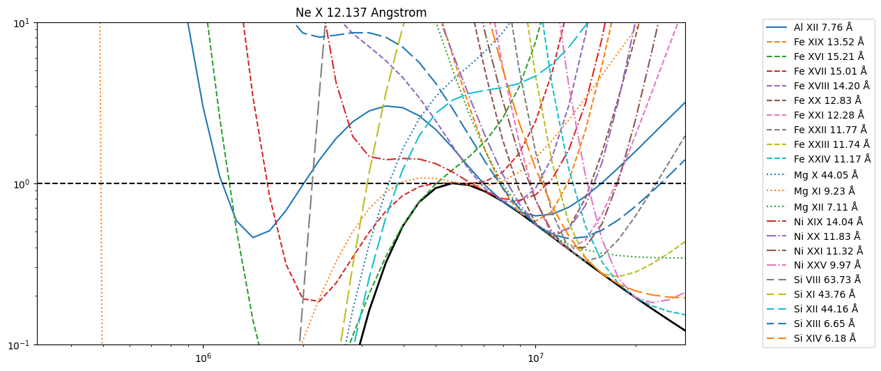

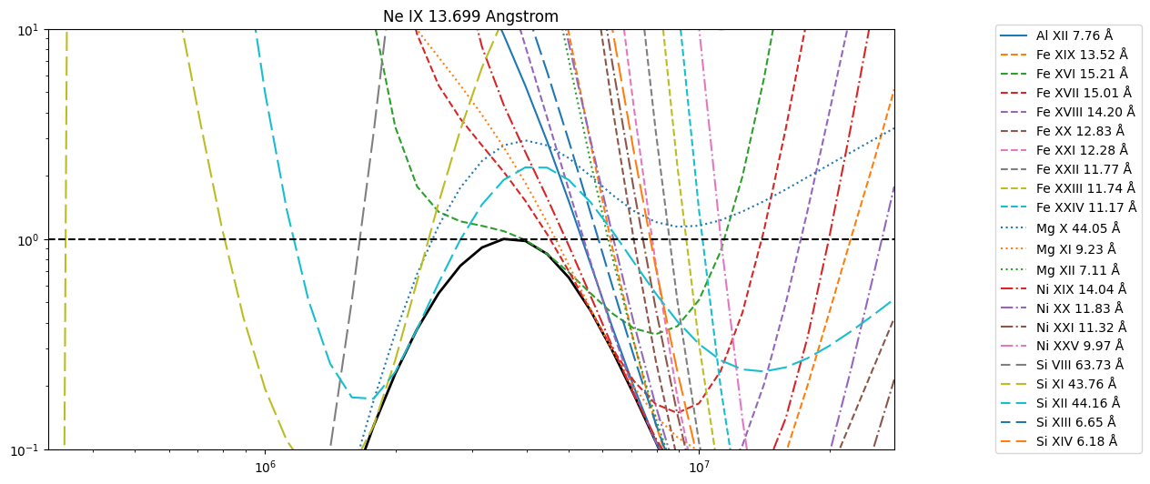
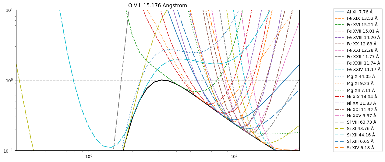
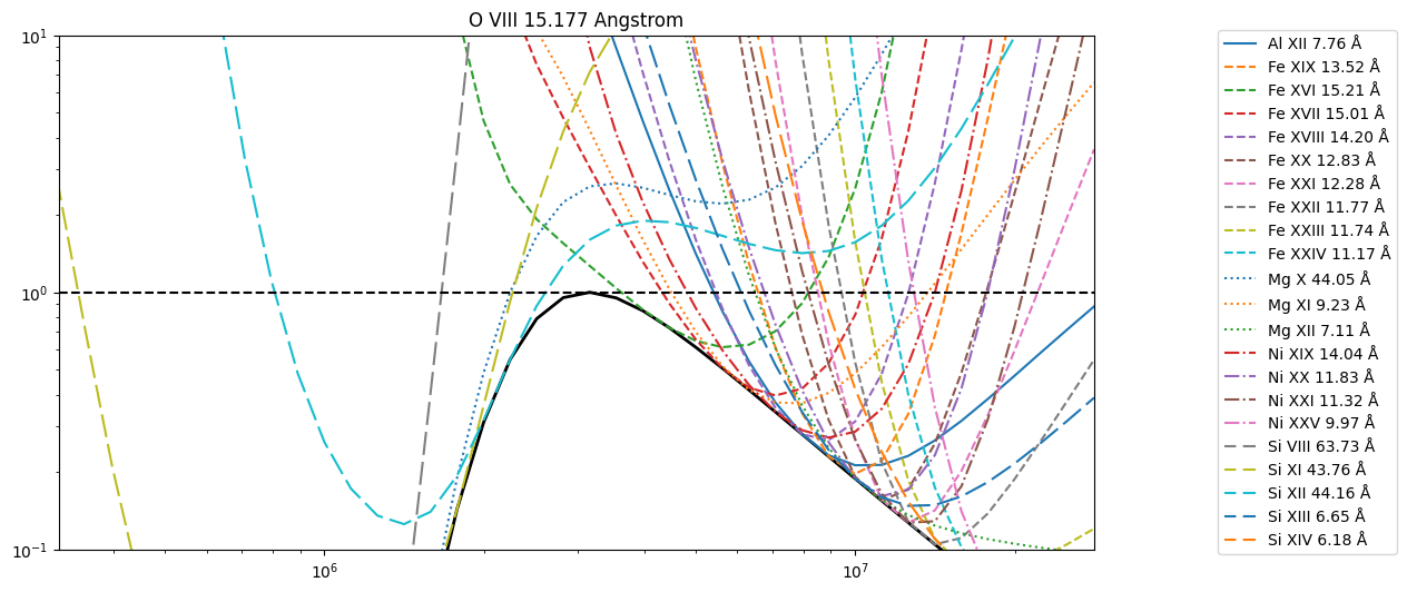

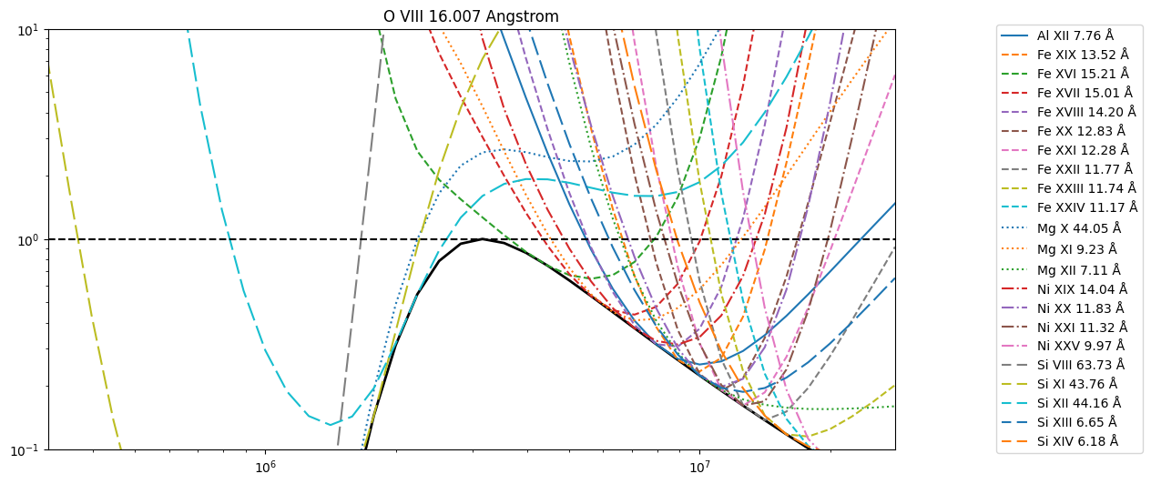
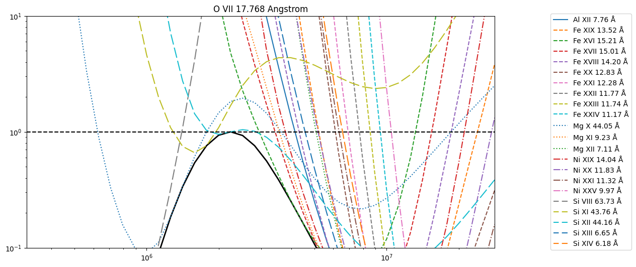
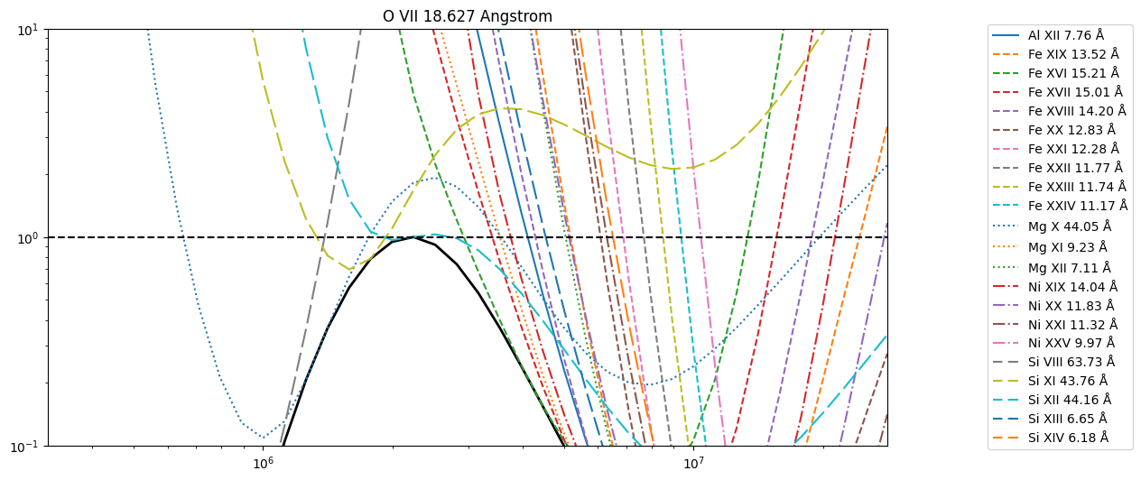
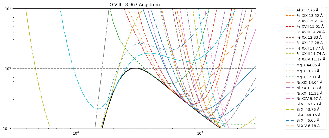
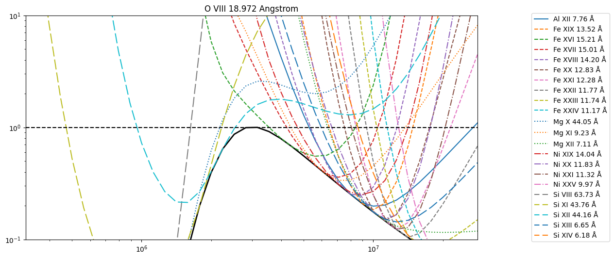
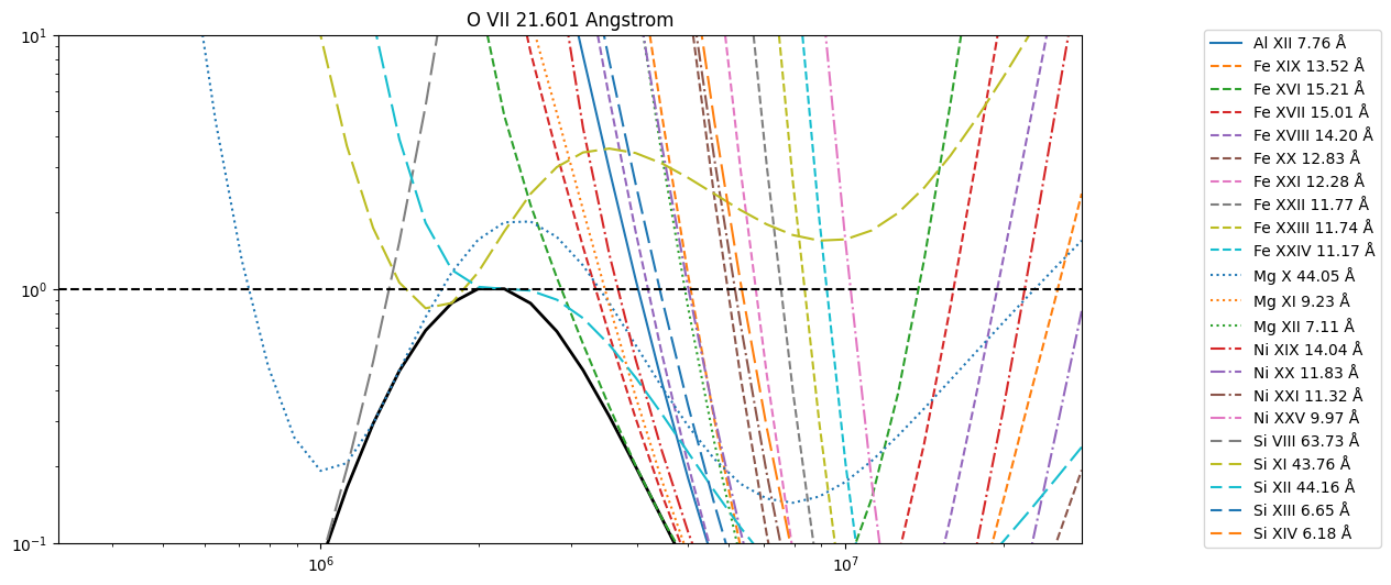
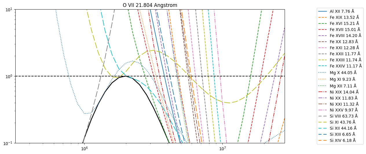
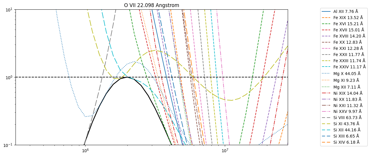
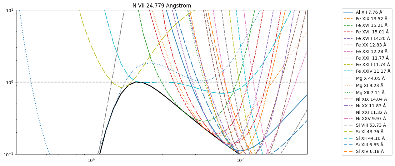
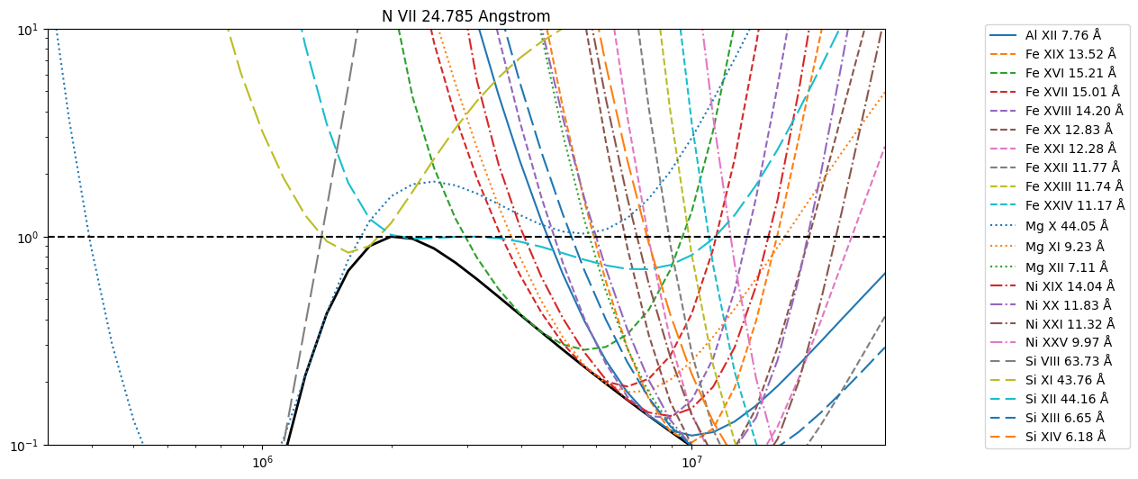
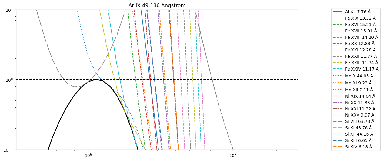
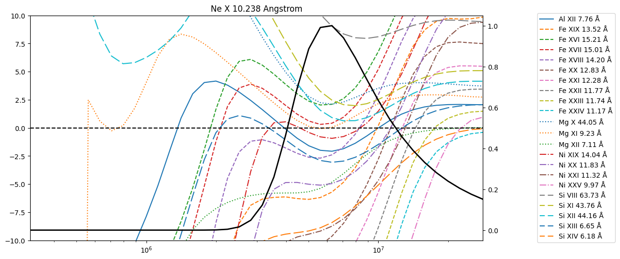
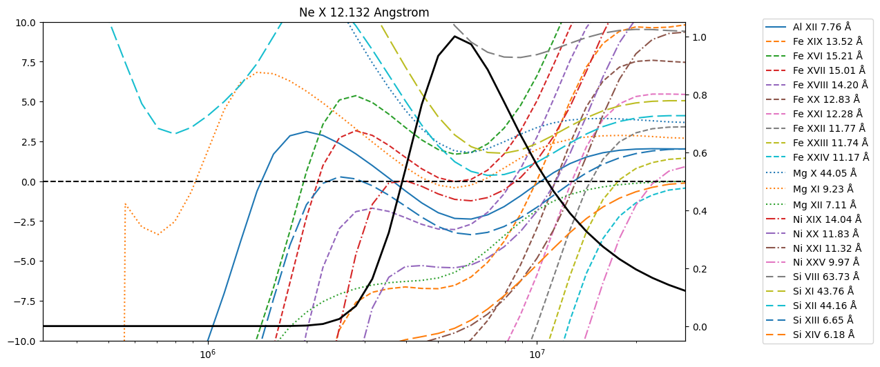
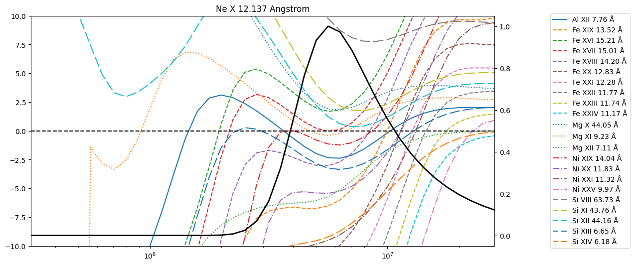
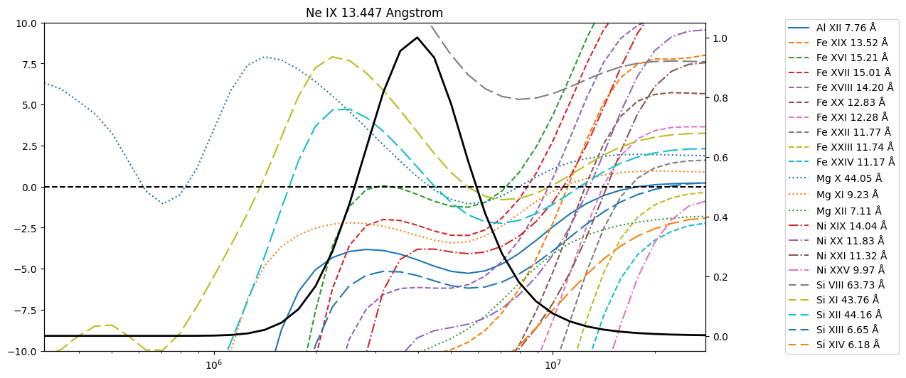
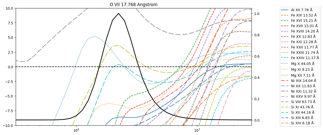
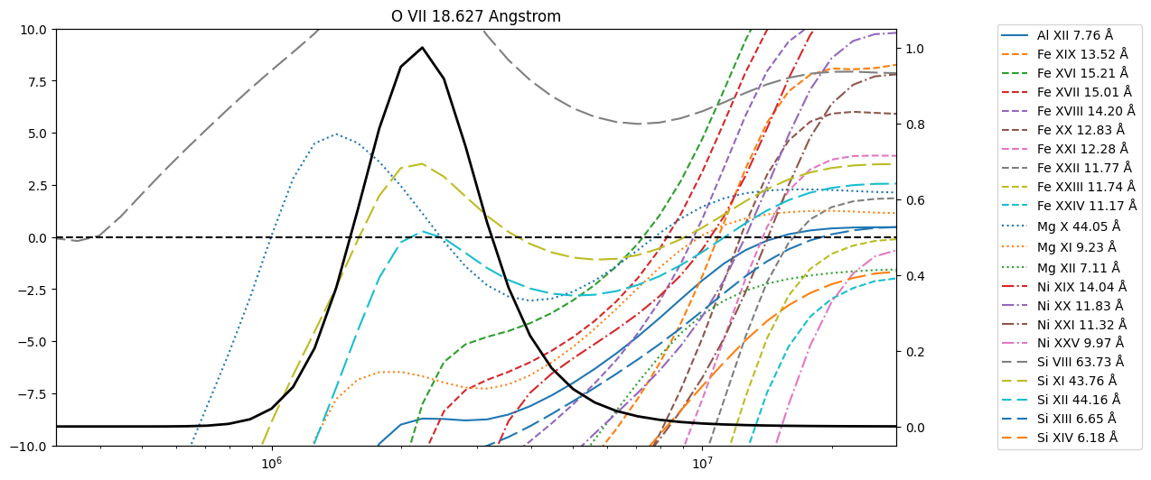
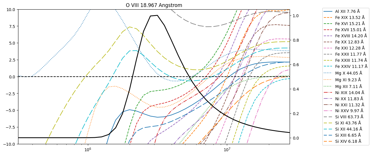
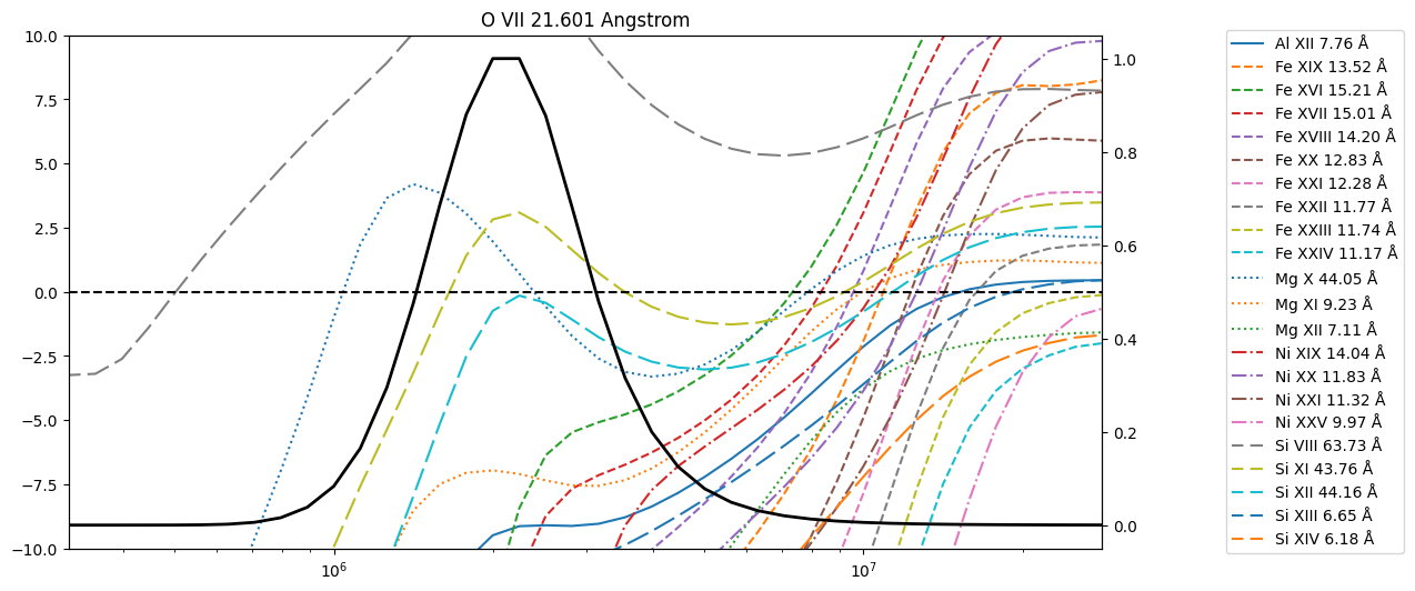
Compute the gradient of this \(G(T)\) ratio. Ideally, the ratio approaches 0 near the peak of the contribution function such that there is little temperature sensitivity near where the lines are strongest and thus any differences when taking a ratio are due to changes in abundance.
[118]:
for hf_row in high_fip_lines:#.group_by('ion name').groups:
    #hf_row = tab[np.argsort(tab['flare\_ext'])][-1]
    goft_hf_strongest = hf_row['contribution function']
    goft_hf_strongest #/= goft_hf_strongest.max()
    #plt.plot(temperature_grid, goft_hf_strongest, label=hf_row['ion name'])
    fig = plt.figure(figsize=(12,6))
    ax = fig.add_subplot()
    ax.set_title(f"{hf_row['ion name']} {hf_row['wavelength']:.3f}")
    ax2 = ax.twinx()
    ax2.plot(temperature_grid, goft_hf_strongest, color='k', lw=2,)
    for tab_lf in low_fip_lines.group_by('ion name').groups:
        lf_row = tab_lf[np.argsort(tab_lf['flare\_ext'])][-1]
        goft_lf_strongest = lf_row['contribution function']
        goft_lf_strongest #/= goft_lf_strongest.max()
        goft_ratio = goft_hf_strongest/goft_lf_strongest
        ax.plot(temperature_grid, np.gradient(np.log10(goft_ratio), np.log10(temperature_grid.value)),#goft_hf_strongest/goft_lf_strongest,
                label=f"{lf_row['ion name']} {lf_row['wavelength'].to_value('Angstrom'):.2f} Å",
                ls=el_linestyles[lf_row['ion name'].split()[0]]['linestyle'])
    #ax.set_yscale('log')
    ax.set_xscale('log')
    #ax.set_ylim(1e-3, 5)
    ax.set_ylim(-10,10)
    ax.set_xlim(temperature_grid[[0,-1]].value)
    ax.axhline(y=0, ls='--', color='k')
    ax.legend(loc='center right', bbox_to_anchor=(1.3,0.5))


Write the table to a format that enables easier reading. This is messy but is a convenient way to render the table as a nicely formatted PDF.
[20]:
import sys
import io
with io.StringIO() as _f:
    flare_snr_table.write(_f,
                          format='ascii.aastex',
                          caption=f'Predicted flare line intensities for MOXSI assuming a source is confined to a single pixel located at disk center at the center of the detector. Lines with an M1 intensity below {threshold:latex_inline} are not included. The flare\\_ext column refers to the CHIANTI flare\\_ext DEM. These intensities are calculated per line. Lines that share a pixel and have flare\\_ext below {max_threshold} of the maximum flare\\_ext in that pixel are also excluded.',
                          #latexdict={'tabletype':'longtable'},
                          formats={
                              'MOXSI pixel': '%d',
                              'wavelength':'%.3f',
                              'energy':'%.3f',
                              '$T_{max}$': '%.1f',
                              '$T_{max,G}$': '%.1f',
                              'IP': '%.1f',
                              r'flare\_ext': '%.3g',
                          #    r'active\_region': '%.3f',
                              **{k.upper(): '%.3f' for k in goes_class}
                          },
                          overwrite=True)
    table_string = _f.getvalue()
md_file = f"""---
title: "MOXSI Flare Lines"
author:
- name: Will Barnes
aastexopts: [singlecolumn]
---

\startlongtable
{table_string}
"""
with open('line-table.md', mode='w') as f:
    f.write(md_file)
!pandoc --template aastex63_template.tex line-table.md -o line-table.pdf
These were the lines that I manually selected based on their relative strength and the criteria that the lines should be reasonably well-separated in first order. Thes critieria were somewhat subjective, but represent a first cut at identifying the lines that have the most diagnostic potential.
[229]:
selected_lines = [
    ('Si XIV        6.180'),
    ('Si XIII       6.648'),
    ('Mg XII        7.106'),
    ('Mg XI 9.231'),
    ('Fe XXI        9.475'),
    ('Fe XIX        9.691'),
    ('Ni XXV        9.967'),
    ('Ne X  10.238'),
    ('Fe XXIV       10.619'),
    ('Fe XXIII      10.980'),
    ('Fe XXIII      11.737'),
    ('Fe XXII       11.767'),
    ('Ni XX 11.832'),
    ('Fe XIX        13.525'),
    ('Fe XX 13.545'),
    ('Ni XIX        14.040'),
    ('Fe XVIII      14.204'),
    ('Fe XVII       15.013'),
    ('Fe XVIII      16.072'),
    ('Fe XVII       17.051'),
    ('O VIII        18.967'),
    ('O VII 21.601'),
    ('N VII 24.779'),
    ('Si XI 43.762'),
    ('Mg X  44.050'),
    ('Si XII        44.160'),
    ('Fe XVI        50.361'),
    ('Si VIII       63.732'),
]
selected_lines = [l.split() for l in selected_lines]
selected_lines = [(f'{l[0]} {l[1]}', float(l[2])*u.AA) for l in selected_lines]
selected_table = []
for ion_name, wavelength in selected_lines:
    _tab = flare_snr_table[flare_snr_table['ion name'] == ion_name]
    _idx = np.argmin(np.fabs(_tab['wavelength']-wavelength))
    selected_table.append(_tab[_idx])
selected_table = astropy.table.vstack(selected_table,)
selected_table.meta = {}
#selected_table
selected_table[['ion name', 'wavelength', 'FIP', 'M1', 'M5', 'X5']].write(
    sys.stdout,
    format='ascii.fixed_width_no_header',
    formats={
        'MOXSI pixel': '%d',
        'wavelength':'%.3f',
        #'energy':'%.3f',
        #'$T_{max}$': '%.1f',
        #r'flare\_ext': '%.3g',
        **{k.upper(): '%.3f' for k in goes_class}
    },
)
WARNING: The key(s) {'MOXSI pixel'} specified in the formats argument do not match a column name. [astropy.io.ascii.ui]
|   Si XIV |  6.180 |  low | 0.191 |  0.773 |   5.959 |
|  Si XIII |  6.648 |  low | 0.389 |  1.699 |  16.016 |
|   Mg XII |  7.106 |  low | 0.166 |  0.718 |   6.601 |
|    Mg XI |  9.231 |  low | 0.326 |  1.380 |  13.309 |
|   Fe XXI |  9.475 |  low | 0.150 |  0.380 |   2.515 |
|   Fe XIX |  9.691 |  low | 0.112 |  0.467 |   4.468 |
|   Ni XXV |  9.967 |  low | 0.131 |  0.572 |   5.512 |
|     Ne X | 10.238 | high | 0.108 |  0.454 |   4.337 |
|  Fe XXIV | 10.619 |  low | 0.152 |  0.717 |   6.446 |
| Fe XXIII | 10.980 |  low | 0.174 |  0.600 |   3.470 |
| Fe XXIII | 11.737 |  low | 0.508 |  1.788 |  10.485 |
|  Fe XXII | 11.767 |  low | 0.176 |  0.422 |   1.695 |
|    Ni XX | 11.832 |  low | 0.105 |  0.437 |   4.166 |
|   Fe XIX | 13.525 |  low | 0.242 |  1.007 |   9.706 |
|    Fe XX | 13.545 |  low | 0.242 |  1.007 |   9.706 |
|   Ni XIX | 14.040 |  low | 0.516 |  2.369 |  23.403 |
| Fe XVIII | 14.204 |  low | 1.501 |  7.086 |  70.478 |
|  Fe XVII | 15.013 |  low | 6.078 | 25.602 | 247.163 |
| Fe XVIII | 16.072 |  low | 0.625 |  2.941 |  29.235 |
|  Fe XVII | 17.051 |  low | 5.158 | 20.753 | 197.723 |
|   O VIII | 18.967 | high | 0.556 |  0.839 |   4.025 |
|    O VII | 21.601 | high | 1.100 |  1.217 |   2.539 |
|    N VII | 24.779 | high | 0.147 |  0.198 |   0.772 |
|    Si XI | 43.762 |  low | 0.104 |  0.138 |   0.522 |
|     Mg X | 44.050 |  low | 0.101 |  0.195 |   1.250 |
|   Si XII | 44.160 |  low | 0.346 |  0.651 |   4.112 |
|   Fe XVI | 50.361 |  low | 0.138 |  0.284 |   1.948 |
|  Si VIII | 63.732 |  low | 0.109 |  0.189 |   1.086 |
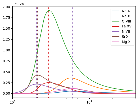
Look at some contribution functions to assess the relative thermal sensitivity of some lines
[125]:
si_13 = fiasco.Ion('Si XIII', np.logspace(5,8,1000)*u.K)
si_12 = fiasco.Ion('Si XII', si_13.temperature)
ne_10 = fiasco.Ion('Ne X', si_13.temperature)
o_8 = fiasco.Ion('O VIII', si_13.temperature)
fe_16 = fiasco.Ion('Fe XVI', si_13.temperature)
fe_17 = fiasco.Ion('Fe XVII', si_13.temperature)
si_11 = fiasco.Ion('Si XI', si_13.temperature)
n_7 = fiasco.Ion('N VII', si_13.temperature)
ni_19 = fiasco.Ion('Ni XIX', si_13.temperature)
mg_11 = fiasco.Ion('Mg XI', si_13.temperature)
[126]:
#goft_si13 = si_13.contribution_function(1e9*u.cm**(-3))
#_idx = np.argmin(np.fabs(si_13.transitions.wavelength[~si_13.transitions.is_twophoton] - 6.6479*u.AA))
#goft_si13 = goft_si13.squeeze()[:,_idx]

goft_si11 = si_11.contribution_function(1e9*u.cm**(-3))
_idx = np.argmin(np.fabs(si_11.transitions.wavelength[~si_11.transitions.is_twophoton] - 49.176*u.AA))
goft_si11 = goft_si11.squeeze()[:,_idx]

goft_n7 = n_7.contribution_function(1e9*u.cm**(-3))
_idx = np.argmin(np.fabs(n_7.transitions.wavelength[~n_7.transitions.is_twophoton] - 24.779*u.AA))
goft_n7 = goft_n7.squeeze()[:,_idx]

goft_ni19 = ni_19.contribution_function(1e9*u.cm**(-3))
_idx = np.argmin(np.fabs(ni_19.transitions.wavelength[~ni_19.transitions.is_twophoton] - 14.040*u.AA))
goft_ni19 = goft_ni19.squeeze()[:,_idx]

# goft_si12 = si_12.contribution_function(1e9*u.cm**(-3))
# _idx = np.argmin(np.fabs(si_12.transitions.wavelength[~si_12.transitions.is_twophoton] - 44.16030*u.AA))
# goft_si12 = goft_si12.squeeze()[:,_idx]

goft_ne10 = ne_10.contribution_function(1e9*u.cm**(-3))
transitions = [10.23849, 12.13210,]*u.AA
_idx = [np.argmin(np.fabs(ne_10.transitions.wavelength[~ne_10.transitions.is_twophoton] - t)) for t in transitions]
goft_ne10 = goft_ne10.squeeze()[:,_idx]

goft_o8 = o_8.contribution_function(1e9*u.cm**(-3))
_idx = np.argmin(np.fabs(o_8.transitions.wavelength[~o_8.transitions.is_twophoton] - 18.9671*u.AA))
goft_o8 = goft_o8.squeeze()[:,_idx]

goft_mg11 = mg_11.contribution_function(1e9*u.cm**(-3))
_idx = np.argmin(np.fabs(mg_11.transitions.wavelength[~mg_11.transitions.is_twophoton] - 9.231*u.AA))
goft_mg11 = goft_mg11.squeeze()[:,_idx]

#goft_fe16 = fe_16.contribution_function(1e9*u.cm**(-3))
#_idx = np.argmin(np.fabs(fe_16.transitions.wavelength[~fe_16.transitions.is_twophoton] - 50.361*u.AA))
#goft_fe16 = goft_fe16.squeeze()[:,_idx]

#goft_fe17 = fe_17.contribution_function(1e9*u.cm**(-3))
#transitions = [15.013, 17.051,]*u.AA
#_idx = [np.argmin(np.fabs(fe_17.transitions.wavelength[~fe_17.transitions.is_twophoton] - t)) for t in transitions]
#goft_fe17 = goft_fe17.squeeze()[:,_idx]
WARNING: No proton data available for N 7. Not including proton excitation and de-excitation in level populations calculation. [fiasco.ions]
WARNING: No proton data available for Ni 19. Not including proton excitation and de-excitation in level populations calculation. [fiasco.ions]
WARNING: No proton data available for Ne 10. Not including proton excitation and de-excitation in level populations calculation. [fiasco.ions]
WARNING: No proton data available for O 8. Not including proton excitation and de-excitation in level populations calculation. [fiasco.ions]
WARNING: No proton data available for Mg 11. Not including proton excitation and de-excitation in level populations calculation. [fiasco.ions]
[134]:
for _ion,_goft in [(ne_10, goft_ne10),
                   (o_8, goft_o8),
                   (fe_16,goft_fe16),
                   #(fe_17, goft_fe17),
                   (n_7, goft_n7),
                   #(si_11,goft_si11),
                   (si_12,goft_si12),
                   #(si_13,goft_si13),
                   #(ni_19,goft_ni19),
                   (mg_11,goft_mg11)]:
    l = plt.plot(_ion.temperature, _goft, label=_ion.ion_name_roman)
    if len(_goft.shape) == 1:
        _goft = _goft[:,np.newaxis]
    for i in range(_goft.shape[1]):
        plt.axvline(x=_ion.temperature[np.argmax(_goft[:,i])].to_value('K'), color=l[i].get_color(), ls=':')

plt.xscale('log')
#plt.yscale('log')
#plt.ylim(1e-27, 8e-24)
plt.xlim(1e6,4e7)
plt.legend()
[134]:
<matplotlib.legend.Legend at 0x356a34510>
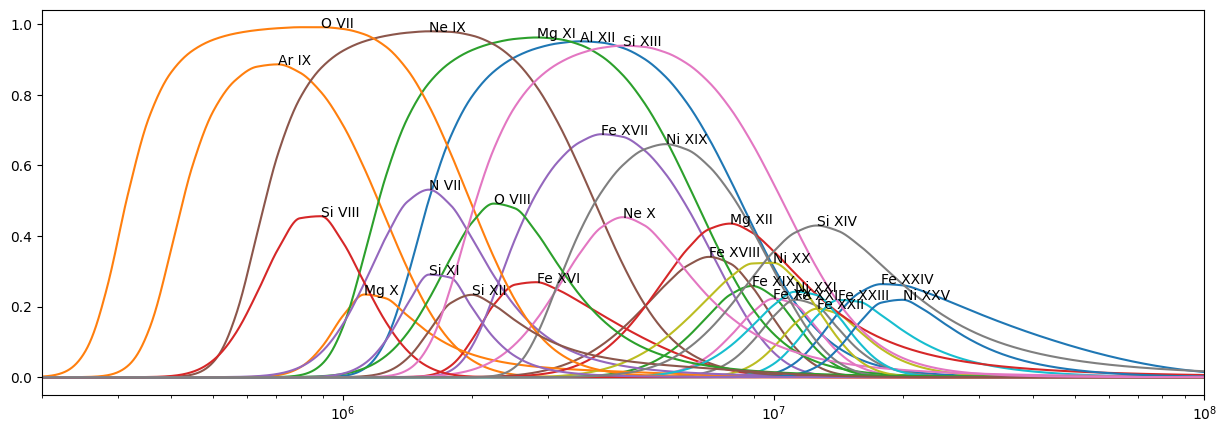
[82]:
ions_unique = np.unique(flare_snr_table['ion name'])
[89]:
fig = plt.figure(figsize=(15,5))
ax = fig.add_subplot()
for i in ions_unique:
    _ion = fiasco.Ion(i, np.logspace(4,8,10000)*u.K)
    ax.plot(_ion.temperature, _ion.ioneq,)
    ax.text(_ion.formation_temperature.value, _ion.ioneq.max(), _ion.ion_name_roman)
plt.xscale('log')
plt.xlim(2e5,1e8)
[89]:
(200000.0, 100000000.0)
How does this compare to our previous curated line list?
[11]:
curated_line_list = astropy.table.QTable.read('../data/line_lists/curated_line_list.asdf')
[12]:
curated_line_list
[12]:
| ion name | wavelength | T_max (Maxwellian) | T_max (kappa=2) | temperature diagnostic | density diagnostic | kappa diagnostic | sass | moxsi | flare line | active region line |
|---|---|---|---|---|---|---|---|---|---|---|
| Angstrom | K | K | ||||||||
| str8 | float64 | float64 | float64 | bool | bool | bool | bool | bool | bool | bool |
| Fe XXV | 1.86 | 31622776.60168379 | 31622776.60168379 | True | False | False | True | False | True | False |
| Ca XIX | 3.21 | 25118864.315095823 | 31622776.60168379 | True | False | False | True | False | True | False |
| Si XIV | 6.1804 | 16185305.906356486 | nan | True | False | False | True | True | True | True |
| Si XIII | 6.74 | 10000000.0 | 12589254.117941663 | True | False | False | True | True | True | False |
| Mg XII | 8.419 | 10000000.0 | 15848931.924611142 | True | False | False | True | True | True | False |
| Mg XI | 9.169 | 6309573.44480193 | 10000000.0 | True | False | False | False | True | True | True |
| Mg XI | 9.314 | 6309573.44480193 | 10000000.0 | True | False | False | False | True | True | True |
| Fe XXIV | 11.171 | 19952623.149688788 | 31622776.60168379 | True | False | False | True | True | True | False |
| Fe XVII | 11.25 | 6309573.44480193 | 7943282.347242822 | True | False | True | False | True | True | True |
| Fe XXIII | 11.737 | 15848931.924611142 | 31622776.60168379 | True | False | False | True | True | True | False |
| Ne X | 12.137 | 6309573.44480193 | 7943282.347242822 | True | False | False | True | True | True | True |
| Fe XX | 12.83 | 10000000.0 | 15848931.924611142 | True | False | False | False | True | True | False |
| Ne IX | 13.447 | 3981071.7055349695 | 5011872.336272725 | True | False | True | False | True | True | True |
| Fe XIX | 13.53 | 10000000.0 | 15848931.924611142 | True | False | False | False | True | True | False |
| Ne IX | 13.669 | 3981071.7055349695 | 5011872.336272725 | True | False | True | False | True | True | True |
| Fe XVIII | 14.204 | 7943282.347242822 | 10000000.0 | True | False | True | False | True | True | True |
| Fe XVII | 15.015 | 6309573.44480193 | 7943282.347242822 | True | False | True | False | True | True | True |
| Fe XVII | 15.25 | 6309573.44480193 | 7943282.347242822 | True | False | True | False | True | True | True |
| O VIII | 16.006 | 3162277.6601683795 | 3981071.7055349695 | True | True | True | False | True | True | True |
| Fe XVII | 16.78 | 6309573.44480193 | 7943282.347242822 | True | False | True | False | True | True | True |
| Fe XVII | 17.05 | 6309573.44480193 | 7943282.347242822 | True | False | True | False | True | True | True |
| Fe XVIII | 17.621 | 7943282.347242822 | 10000000.0 | True | False | True | False | True | True | True |
| O VII | 18.67 | 1995262.3149688789 | 2511886.4315095823 | True | True | True | False | True | True | True |
| O VIII | 18.967 | 3162277.6601683795 | 3981071.7055349695 | True | True | True | False | True | True | True |
| O VII | 21.6 | 1995262.3149688789 | 2511886.4315095823 | True | True | True | False | True | True | True |
| O VII | 21.81 | 1995262.3149688789 | 2511886.4315095823 | True | True | True | False | True | True | True |
| O VII | 22.1 | 1995262.3149688789 | 2511886.4315095823 | True | True | True | False | True | True | True |
| N VII | 24.77 | 1995262.3149688789 | 3162277.6601683795 | True | False | False | False | True | True | True |
| C VI | 33.73 | 1258925.411794166 | 1995262.3149688789 | True | False | False | False | True | False | True |
| C V | 40.27 | 1000000.0 | 1258925.411794166 | True | False | False | False | True | False | True |
| Si XII | 44.16 | 1995262.3149688789 | 3162277.6601683795 | True | False | False | False | True | True | True |
| Si XI | 49.18 | 1584893.1924611141 | 1995262.3149688789 | True | False | False | False | True | False | True |
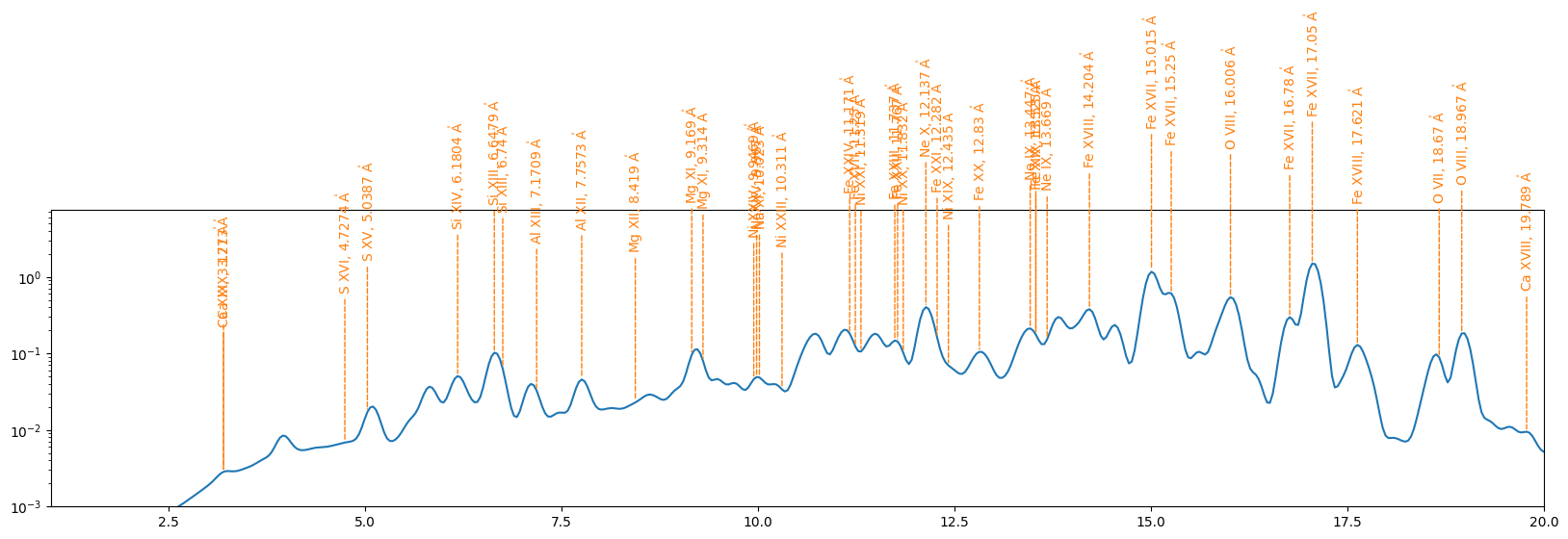
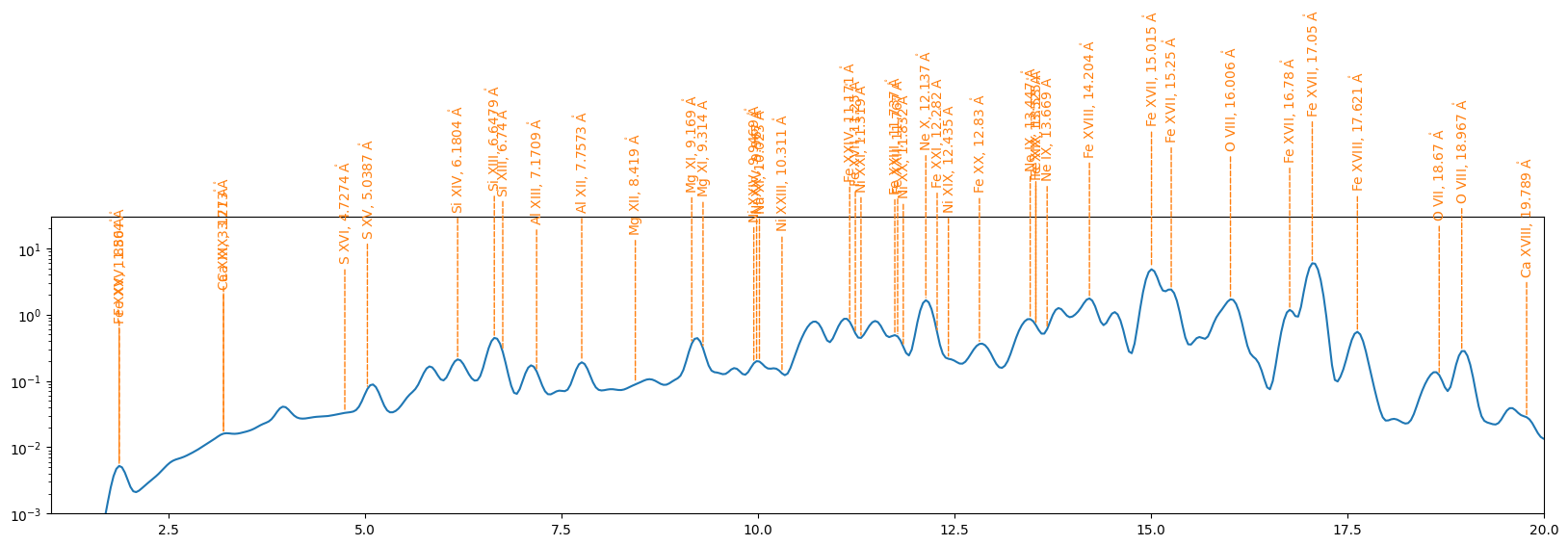
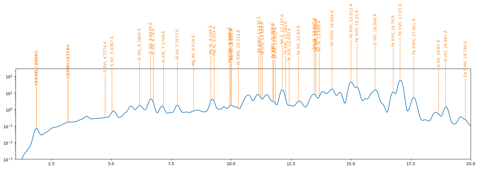
Do some visual checks
[20]:
blur = 40 * u.arcsec
[25]:
for gc in goes_class:
    fig = plt.figure(figsize=(20,4))
    ax = fig.add_subplot()
    flux = convolve_with_response(flare_spectra[gc], channel_o1, electrons=False, include_gain=False)
    flux = _blur_spectra(flux, blur / channel_o1.spatial_plate_scale[0] * channel_o1.spectral_plate_scale, channel_o1)
    ax.plot(flux.axis_world_coords(0)[0], flux.data)
    annotate_lines(ax, combined_line_list, flux, 'C1', rtol=0.0)
    ax.set_yscale('log')
    ax.set_xlim(1,20)
    ax.set_ylim(1e-3,flux.data.max()*5)
[ ]: