Lossless JPEG Experimentation#
Question: how effective is JPEG-LS at compressing our 1 second exposures?
This notebook compares the effectiveness of JPEG-LS compared to JPEG and JPEG-2000 for several simple parameterizations. The relevant metric here is just the ratio of the file size between the JPEG-LS files compared to other formats.
[330]:
import pathlib
import tempfile

import numpy as np
import matplotlib.pyplot as plt
from astropy.visualization import ImageNormalize, LogStretch, AsymmetricPercentileInterval
import astropy.units as u

import PIL
import pillow_jpls

from overlappy.util import color_lat_lon_axes
from mocksipipeline.util import stack_components
[435]:
def compare_jpeg_ls_compression(array, compare_format='JPEG2000', mode='I;16'):
    pil_image = PIL.Image.fromarray(array.astype(np.uint16)).convert(mode=mode)
    with tempfile.TemporaryDirectory() as tmpdir:
        tmpdir_p = pathlib.Path(tmpdir)
        jpls_path = tmpdir_p / 'image.jls'
        jp_path = tmpdir_p / 'image.jpg'
        pil_image.save(jpls_path, format='JPEG-LS')
        jpeg_ls_size = jpls_path.stat().st_size * u.byte
        print('JPEG-LS size: ',jpeg_ls_size.to('kilobyte'))
        if compare_format is None:
            other_size = np.product(array.shape) * 16 * u.bit
        else:
            pil_image.save(jp_path, format=compare_format)
            other_size = jp_path.stat().st_size * u.byte
        print('Other size: ',other_size.to('kilobyte'))
        ratio = other_size / jpeg_ls_size

    return ratio.decompose()
[390]:
data_dir = pathlib.Path('data/')
[391]:
files = data_dir.glob('overlappogram-ar-photons-order=*.fits')
[392]:
overlappogram = stack_components(sorted(files), wcs_index=2)
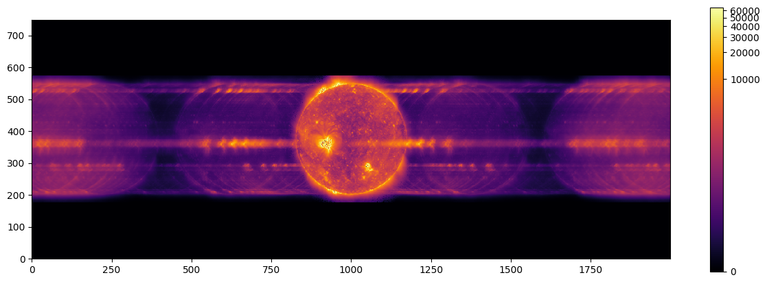
[393]:
fig = plt.figure(figsize=(15,5))
vmin,vmax = AsymmetricPercentileInterval(1,99.9).get_limits(overlappogram[0].data)
#vmin,vmax = None, None
norm = ImageNormalize(vmin=vmin, vmax=vmax, stretch=LogStretch())
ax = fig.add_subplot(projection=overlappogram[0].wcs)
overlappogram[0].plot(
    axes=ax,
    norm=norm,
    data_unit='photon / (pix s)',
    cmap='viridis',
)
color_lat_lon_axes(ax)
plt.colorbar()
[393]:
<matplotlib.colorbar.Colorbar at 0x7fc568ac7370>

Everything is 1#
[394]:
overlappogram_ones = np.ones(overlappogram.data[0].shape)
[395]:
plt.figure(figsize=(15,5))
vmin, vmax = AsymmetricPercentileInterval(0,100).get_limits(overlappogram_random)
plt.imshow(overlappogram_ones,
           origin='lower', norm=ImageNormalize(vmin=vmin, vmax=vmax, stretch=LogStretch()), interpolation='none', cmap='inferno')
plt.colorbar()
[395]:
<matplotlib.colorbar.Colorbar at 0x7fc5689c20b0>
[436]:
compare_jpeg_ls_compression(overlappogram_ones, compare_format='JPEG', mode='L')
JPEG-LS size:  0.443 kbyte
Other size:  17.957 kbyte
[436]:
[437]:
compare_jpeg_ls_compression(overlappogram_ones, compare_format='JPEG2000', mode='I;16')
JPEG-LS size:  0.544 kbyte
Other size:  0.23700000000000002 kbyte
[437]:
[438]:
compare_jpeg_ls_compression(overlappogram_ones, compare_format=None, mode='I;16')
JPEG-LS size:  0.544 kbyte
Other size:  3000.0 kbyte
[438]:
Everything is 0#
[399]:
overlappogram_zeros = np.zeros(overlappogram.data[0].shape)
[400]:
plt.figure(figsize=(15,5))
vmin, vmax = AsymmetricPercentileInterval(0,100).get_limits(overlappogram_random)
plt.imshow(overlappogram_zeros,
           origin='lower', norm=ImageNormalize(vmin=vmin, vmax=vmax, stretch=LogStretch()), interpolation='none', cmap='inferno')
plt.colorbar()
[400]:
<matplotlib.colorbar.Colorbar at 0x7fc5688a3430>
[439]:
compare_jpeg_ls_compression(overlappogram_zeros, compare_format='JPEG', mode='L')
JPEG-LS size:  0.17500000000000002 kbyte
Other size:  17.957 kbyte
[439]:
[440]:
compare_jpeg_ls_compression(overlappogram_zeros, compare_format='JPEG2000', mode='I;16')
JPEG-LS size:  0.19 kbyte
Other size:  0.23800000000000002 kbyte
[440]:
[441]:
compare_jpeg_ls_compression(overlappogram_zeros, compare_format=None, mode='I;16')
JPEG-LS size:  0.19 kbyte
Other size:  3000.0 kbyte
[441]:
Random Counts#
Random distribution of counts over the detector
[404]:
overlappogram_random = np.random.randint(0, high=5, size=overlappogram.data[0].shape, dtype=np.uint16)
[405]:
plt.figure(figsize=(15,5))
vmin, vmax = AsymmetricPercentileInterval(0,100).get_limits(overlappogram_random)
plt.imshow(overlappogram_random,
           origin='lower', norm=ImageNormalize(vmin=vmin, vmax=vmax, stretch=LogStretch()), interpolation='none', cmap='inferno')
plt.colorbar()
[405]:
<matplotlib.colorbar.Colorbar at 0x7fc56879ece0>

[442]:
compare_jpeg_ls_compression(overlappogram_random, compare_format='JPEG', mode='L')
JPEG-LS size:  538.343 kbyte
Other size:  23.185 kbyte
[442]:
[443]:
compare_jpeg_ls_compression(overlappogram_random, compare_format='JPEG2000', mode='I;16')
JPEG-LS size:  546.984 kbyte
Other size:  535.896 kbyte
[443]:
[444]:
compare_jpeg_ls_compression(overlappogram_random, compare_format=None, mode='I;16')
JPEG-LS size:  546.984 kbyte
Other size:  3000.0 kbyte
[444]:
Thresholding non-zero values#
This just makes everything over some threshold value 1 and everything else 0
[409]:
overlappogram_bool = (overlappogram.data[0] > 0.001).astype(np.uint16)
[410]:
plt.figure(figsize=(15,5))
vmin, vmax = AsymmetricPercentileInterval(0,100).get_limits(overlappogram_bool)
plt.imshow(overlappogram_bool,
           origin='lower', norm=ImageNormalize(vmin=vmin, vmax=vmax, stretch=LogStretch()), interpolation='none', cmap='inferno')
plt.colorbar()
[410]:
<matplotlib.colorbar.Colorbar at 0x7fc568671e10>

[445]:
compare_jpeg_ls_compression(overlappogram_bool, compare_format='JPEG', mode='L')
JPEG-LS size:  5.287 kbyte
Other size:  18.046 kbyte
[445]:
[446]:
compare_jpeg_ls_compression(overlappogram_bool, compare_format='JPEG2000', mode='I;16')
JPEG-LS size:  6.008 kbyte
Other size:  7.162 kbyte
[446]:
[447]:
compare_jpeg_ls_compression(overlappogram_bool, compare_format=None, mode='I;16')
JPEG-LS size:  6.008 kbyte
Other size:  3000.0 kbyte
[447]:
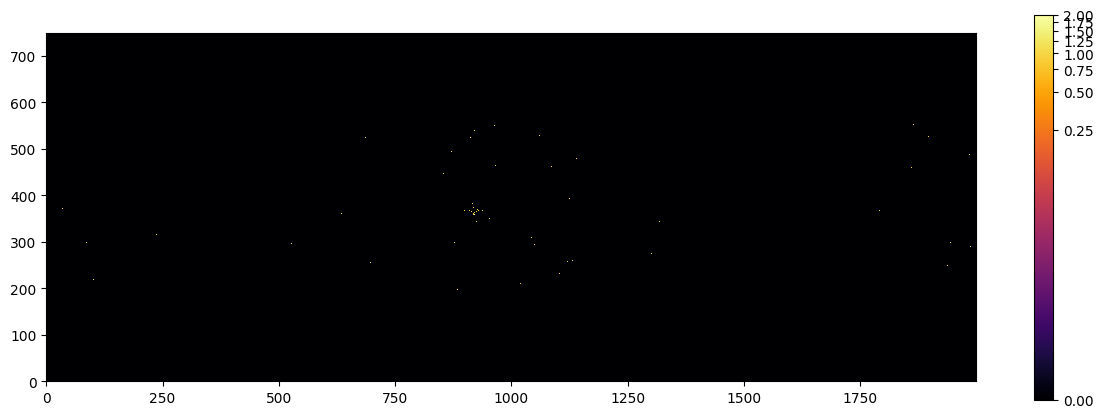
Sampling from a Poisson Distribution#
Use the simulated image create a Poisson distribution for each pixel.
[448]:
dt = 1 * u.s
[449]:
probability_rate = overlappogram[0].data * overlappogram.unit * u.pix
[450]:
counts = np.random.poisson(lam=(probability_rate*dt).to_value('photon'))
[451]:
counts
[451]:
array([[0, 0, 0, ..., 0, 0, 0],
       [0, 0, 0, ..., 0, 0, 0],
       [0, 0, 0, ..., 0, 0, 0],
       ...,
       [0, 0, 0, ..., 0, 0, 0],
       [0, 0, 0, ..., 0, 0, 0],
       [0, 0, 0, ..., 0, 0, 0]])
[452]:
plt.figure(figsize=(15,5))
vmin, vmax = AsymmetricPercentileInterval(0,100).get_limits(counts)
plt.imshow(counts,
           origin='lower', norm=ImageNormalize(vmin=vmin, vmax=vmax, stretch=LogStretch()), interpolation='none', cmap='inferno')
plt.colorbar()
[452]:
<matplotlib.colorbar.Colorbar at 0x7fc5684077f0>
[453]:
compare_jpeg_ls_compression(counts, compare_format='JPEG', mode='L')
JPEG-LS size:  0.589 kbyte
Other size:  17.957 kbyte
[453]:
[454]:
compare_jpeg_ls_compression(counts, compare_format='JPEG2000', mode='I;16')
JPEG-LS size:  0.81 kbyte
Other size:  1.0110000000000001 kbyte
[454]:
[455]:
compare_jpeg_ls_compression(counts, compare_format=None, mode='I;16')
JPEG-LS size:  0.81 kbyte
Other size:  3000.0 kbyte
[455]:
Scaling Up the Overlappogram Image#
[456]:
scaling_factor = 1 / overlappogram.data[0][np.nonzero(overlappogram.data[0])].min()
[457]:
overlappogram_scaled = (overlappogram.data[0] * scaling_factor).astype(np.uint16)
[458]:
plt.figure(figsize=(15,5))
vmin, vmax = AsymmetricPercentileInterval(0,100).get_limits(overlappogram_scaled)
plt.imshow(overlappogram_scaled,
           origin='lower', norm=ImageNormalize(vmin=vmin, vmax=vmax, stretch=LogStretch()), interpolation='none', cmap='inferno')
plt.colorbar()
[458]:
<matplotlib.colorbar.Colorbar at 0x7fc568378f10>
[459]:
compare_jpeg_ls_compression(overlappogram_scaled, compare_format='JPEG', mode='L')
JPEG-LS size:  148.861 kbyte
Other size:  63.115 kbyte
[459]:
[460]:
compare_jpeg_ls_compression(overlappogram_scaled, compare_format='JPEG2000', mode='I;16')
JPEG-LS size:  601.905 kbyte
Other size:  607.489 kbyte
[460]:
[461]:
compare_jpeg_ls_compression(overlappogram_scaled, compare_format=None, mode='I;16')
JPEG-LS size:  601.905 kbyte
Other size:  3000.0 kbyte
[461]:
Conclusions#
JPEG2000 and JPEG-LS provide similar compression in nearly all cases
JPEG-LS provides marginally better performance (factor of \(\approx1.2\)) than JPEG2000 for Poisson sampling case
The noiser the image, the worse JPEG-LS does compared to normal JPEG–see uniform distribution case above
The more areas of continuous tone the better the performance
More zeros perform better than more non-zeros
JPEG-LS provides a factor of \(\approx30\) better compression than JPEG for most realistic case of Poisson sampling
The more photons we have, the worse JPEG-LS will do
[ ]: