Assessing line diagnostics for different tube lengths#

Need to understand what we’re losing by shortening the tube and losing wavelengths

[145]:

import copy

import astropy.table
import astropy.units as u
import matplotlib.pyplot as plt
from adjustText import adjust_text
import numpy as np
import fiasco
from scipy.interpolate import interp1d
from aiapy.response import Channel

from astropy.visualization import quantity_support

from mocksipipeline.detector.response import SpectrogramChannel

[3]:

line_list = astropy.table.QTable.read('../data/line_lists/curated_line_list.asdf')

WARNING: UnitsWarning: The unit 'Angstrom' has been deprecated in the VOUnit standard. Suggested: 0.1nm. [astropy.units.format.utils]

[8]:

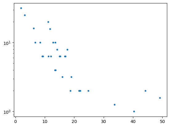
plt.plot(line_list['wavelength'], line_list['T_max (Maxwellian)'].to('MK'),
         marker='.', ls='')
plt.yscale('log')

../_images/reports_temperature-wave-space_3_0.png

[257]:

full_line_list = astropy.table.QTable.read('../data/line_lists/full-line-list.asdf')

WARNING: UnitsWarning: The unit 'Angstrom' has been deprecated in the VOUnit standard. Suggested: 0.1nm. [astropy.units.format.utils]

[258]:

channel_o1 = SpectrogramChannel(1)

[259]:

response_unit = u.Unit('cm2 sr / ( pix)')
intensity_unit = response_unit * u.Unit('ph cm-2 s-1 sr-1')
f_interp_ea = interp1d(channel_o1.wavelength.to_value('AA'),
                       (channel_o1.effective_area* channel_o1.plate_scale).to_value(response_unit),
                       bounds_error=True,
                       assume_sorted=False)
plt.plot(full_line_list['wavelength'], f_interp_ea(full_line_list['wavelength'].to_value('AA')), marker='.', ls='')
plt.plot(channel_o1.wavelength, channel_o1.effective_area*channel_o1.plate_scale)
plt.yscale('log')

/Users/wtbarnes/mambaforge/envs/mocksipipeline/lib/python3.9/site-packages/astropy/units/quantity.py:673: RuntimeWarning: divide by zero encountered in divide
  result = super().__array_ufunc__(function, method, *arrays, **kwargs)

../_images/reports_temperature-wave-space_6_1.png

[260]:

# Add a T_max column based on the ionization fraction (existing ones depend on the DEM used)
temperature_grid = 10**np.arange(4,8,0.001)*u.K
all_chianti_ions = [fiasco.Ion(i, temperature_grid) for i in fiasco.list_ions(fiasco.defaults['hdf5_dbase_root'])]
ioneq_tmax = {i.ion_name_roman: i.formation_temperature for i in all_chianti_ions}
#full_line_list['T_max (Maxwellian)'] = list(map(lambda x: ioneq_tmax[x], full_line_list['ion name']))
# Add a FIP column
all_chianti_elements = [fiasco.Element(el, 1*u.MK) for el in fiasco.list_elements(fiasco.defaults['hdf5_dbase_root'])]
element_is_low_fip = {el.atomic_symbol: el[0].ip<=10*u.eV for el in all_chianti_elements}
full_line_list['is low FIP'] = list(map(lambda x: element_is_low_fip[x], full_line_list['element']))
# Add a column that expresses the intensity in MOXSI detector units
full_line_list['intensity_moxsi (coronal)_active_region'] = (full_line_list['intensity (coronal)_active_region']
                                                             * f_interp_ea(full_line_list['wavelength'].to_value('AA'))
                                                             * u.Unit(response_unit)).to(intensity_unit)
full_line_list['intensity_moxsi_scaled (coronal)_active_region'] = full_line_list['intensity_moxsi (coronal)_active_region'] / full_line_list['intensity_moxsi (coronal)_active_region'].max()
full_line_list['intensity_moxsi (coronal)_flare_ext'] = (full_line_list['intensity (coronal)_flare_ext']
                                                         * f_interp_ea(full_line_list['wavelength'].to_value('AA'))
                                                         * u.Unit(response_unit)).to(intensity_unit)
full_line_list['intensity_moxsi_scaled (coronal)_flare_ext'] = full_line_list['intensity_moxsi (coronal)_flare_ext'] / full_line_list['intensity_moxsi (coronal)_flare_ext'].max()

[263]:

full_line_list.colnames

[263]:

['atomic number',
 'ionization stage',
 'transition',
 'transition (latex)',
 'ion name',
 'lower level',
 'upper level',
 'max temperature_flare_ext',
 'wavelength',
 'only theoretical_flare_ext',
 'element',
 'ion id',
 'energy',
 'abundance (coronal)',
 'abundance (photospheric)',
 'intensity (coronal)_flare_ext',
 'intensity_scaled (coronal)_flare_ext',
 'intensity (photospheric)_flare_ext',
 'intensity_scaled (photospheric)_flare_ext',
 'max temperature_active_region',
 'only theoretical_active_region',
 'intensity (coronal)_active_region',
 'intensity_scaled (coronal)_active_region',
 'intensity (photospheric)_active_region',
 'intensity_scaled (photospheric)_active_region',
 'is low FIP',
 'intensity_moxsi (coronal)_active_region',
 'intensity_moxsi_scaled (coronal)_active_region',
 'intensity_moxsi (coronal)_flare_ext',
 'intensity_moxsi_scaled (coronal)_flare_ext']

[315]:

fig = plt.figure(figsize=(18,10))
ax = fig.add_subplot(111)
low_fip_color = 'C5'
high_fip_color = 'C6'
with quantity_support():
    ax.scatter(full_line_list['wavelength'],
               full_line_list['max temperature_active_region'].to('MK'),
               s=full_line_list['intensity_scaled (coronal)_active_region']*3e3,
               marker='.', alpha=0.3, color=[low_fip_color if r['is low FIP'] else high_fip_color for r in full_line_list])
    for ls,spec_res in zip(['--', ':'], [55, 71.8] * u.milliAA / u.pix):
        max_wave = 1000 * u.pix * spec_res
        for i,order in enumerate([1,2,3,4]):
            ax.axvline(x=max_wave/order, ls=ls, color=f'C{i}')
    ax.axhline(y=1*u.MK, ls='-.', color='k', lw=1)
    ax.axhline(y=10*u.MK, ls='-.', color='k', lw=1)

    line_labels = []
    line_label_tol = 0.05
    for row in full_line_list:
        if row['intensity_scaled (coronal)_active_region'] >= line_label_tol:
            line_labels.append(ax.text(row['wavelength'], row['max temperature_active_region'], row['ion name'],
                                       color=low_fip_color if row['is low FIP'] else high_fip_color))
    adjust_text(
        line_labels,
        x=copy.deepcopy(full_line_list['wavelength'].to_value('AA')),
        y=copy.deepcopy(full_line_list['max temperature_active_region'].to_value('MK')),
        avoid_points=False,
        arrowprops=dict(arrowstyle='->', color='k', alpha=0.75),
    )
    #ax.set_yscale('log')
    ax.set_ylim(0,10.1)
    ax.set_title('AR Intensities')
    ax.legend(handles=[plt.Line2D([0], [0], marker='.', color=low_fip_color, label='Low FIP', ls='', alpha=0.3, markersize=15),
                       plt.Line2D([0], [0], marker='.', color=high_fip_color, label='High FIP', ls='', alpha=0.3, markersize=15)],
              loc=1, frameon=False)
ax.set_xlabel(r'Transition Wavelength [Å]')
ax.set_ylabel(r'Effective Formation Temperature ($\argmax_T G(T)\mathrm{DEM}(T)$) [MK]')

[315]:

Text(192.09722222222223, 0.5, 'Effective Formation Temperature ($\\argmax_T G(T)\\mathrm{DEM}(T)$) [MK]')

../_images/reports_temperature-wave-space_9_1.png

[319]:

fig = plt.figure(figsize=(18,10))
ax = fig.add_subplot(111)
low_fip_color = 'C5'
high_fip_color = 'C6'
with quantity_support():
    ax.scatter(full_line_list['wavelength'],
               full_line_list['max temperature_active_region'].to('MK'),
               s=full_line_list['intensity_moxsi_scaled (coronal)_active_region']*3e3,
               marker='.', alpha=0.3, color=[low_fip_color if r['is low FIP'] else high_fip_color for r in full_line_list])
    for ls,spec_res in zip(['--', ':'], [55, 71.8] * u.milliAA / u.pix):
        max_wave = 1000 * u.pix * spec_res
        for i,order in enumerate([1,2,3,4]):
            ax.axvline(x=max_wave/order, ls=ls, color=f'C{i}')
    ax.axhline(y=1*u.MK, ls='-.', color='k', lw=1)
    ax.axhline(y=10*u.MK, ls='-.', color='k', lw=1)

    line_labels = []
    line_label_tol = 0.01
    for row in full_line_list:
        if row['intensity_moxsi_scaled (coronal)_active_region'] >= line_label_tol:
            line_labels.append(ax.text(row['wavelength'], row['max temperature_active_region'], row['ion name'],
                                       color=low_fip_color if row['is low FIP'] else high_fip_color))
    adjust_text(
        line_labels,
        x=copy.deepcopy(full_line_list['wavelength'].to_value('AA')),
        y=copy.deepcopy(full_line_list['max temperature_active_region'].to_value('MK')),
        avoid_points=False,
        arrowprops=dict(arrowstyle='->', color='k', alpha=0.75),
    )
    #ax.set_yscale('log')
    ax.set_ylim(0,10.1)
    ax.set_title('AR Intensities')
    ax.legend(handles=[plt.Line2D([0], [0], marker='.', color=low_fip_color, label='Low FIP', ls='', alpha=0.3, markersize=15),
                       plt.Line2D([0], [0], marker='.', color=high_fip_color, label='High FIP', ls='', alpha=0.3, markersize=15)],
              loc=1, frameon=False)
ax.set_xlabel(r'Transition Wavelength [Å]')
ax.set_ylabel(r'Effective Formation Temperature ($\argmax_T G(T)\mathrm{DEM}(T)$) [MK]')

[319]:

Text(192.09722222222223, 0.5, 'Effective Formation Temperature ($\\argmax_T G(T)\\mathrm{DEM}(T)$) [MK]')

../_images/reports_temperature-wave-space_10_1.png

[321]:

fig = plt.figure(figsize=(18,10))
ax = fig.add_subplot(111)
with quantity_support():
    ax.scatter(full_line_list['wavelength'],
               full_line_list['max temperature_flare_ext'].to('MK'),
               s=full_line_list['intensity_scaled (coronal)_flare_ext']*3e3,
               marker='.', alpha=0.3, color=[low_fip_color if r['is low FIP'] else high_fip_color for r in full_line_list])
    for ls,spec_res in zip(['--', ':'], [55, 71.8] * u.milliAA / u.pix):
        max_wave = 1000 * u.pix * spec_res
        for i,order in enumerate([1,2,3,4]):
            ax.axvline(x=max_wave/order, ls=ls, color=f'C{i}')
    ax.axhline(y=1*u.MK, ls='-.', color='k', lw=1)
    ax.axhline(y=10*u.MK, ls='-.', color='k', lw=1)

    line_labels = []
    line_label_tol = 0.03
    for row in full_line_list:
        if row['intensity_scaled (coronal)_flare_ext'] >= line_label_tol:
            line_labels.append(ax.text(row['wavelength'], row['max temperature_flare_ext'], row['ion name'],
                                       color=low_fip_color if row['is low FIP'] else high_fip_color,clip_on=True))
    adjust_text(
        line_labels,
        x=copy.deepcopy(full_line_list['wavelength'].to_value('AA')),
        y=copy.deepcopy(full_line_list['max temperature_flare_ext'].to_value('MK')),
        avoid_points=False,
        arrowprops=dict(arrowstyle='->', color='k', alpha=0.75),
        clip_on=True,
    )
    #ax.set_yscale('log')
    ax.set_ylim(0,40)
    ax.set_title('Flare Intensities')
    ax.legend(handles=[plt.Line2D([0], [0], marker='.', color=low_fip_color, label='Low FIP', ls='', alpha=0.3, markersize=15),
                   plt.Line2D([0], [0], marker='.', color=high_fip_color, label='High FIP', ls='', alpha=0.3, markersize=15)],
          loc=1, frameon=False)
ax.set_xlabel(r'Transition Wavelength [Å]')
ax.set_ylabel(r'Effective Formation Temperature ($\argmax_T G(T)\mathrm{DEM}(T)$) [MK]')

[321]:

Text(192.09722222222223, 0.5, 'Effective Formation Temperature ($\\argmax_T G(T)\\mathrm{DEM}(T)$) [MK]')

../_images/reports_temperature-wave-space_11_1.png

[320]:

fig = plt.figure(figsize=(18,10))
ax = fig.add_subplot(111)
with quantity_support():
    ax.scatter(full_line_list['wavelength'],
               full_line_list['max temperature_flare_ext'].to('MK'),
               s=full_line_list['intensity_moxsi_scaled (coronal)_flare_ext']*3e3,
               marker='.', alpha=0.3, color=[low_fip_color if r['is low FIP'] else high_fip_color for r in full_line_list])
    for ls,spec_res in zip(['--', ':'], [55, 71.8] * u.milliAA / u.pix):
        max_wave = 1000 * u.pix * spec_res
        for i,order in enumerate([1,2,3,4]):
            ax.axvline(x=max_wave/order, ls=ls, color=f'C{i}')
    ax.axhline(y=1*u.MK, ls='-.', color='k', lw=1)
    ax.axhline(y=10*u.MK, ls='-.', color='k', lw=1)

    line_labels = []
    line_label_tol = 0.03
    for row in full_line_list:
        if row['intensity_moxsi_scaled (coronal)_flare_ext'] >= line_label_tol:
            line_labels.append(ax.text(row['wavelength'], row['max temperature_flare_ext'], row['ion name'],
                                       color=low_fip_color if row['is low FIP'] else high_fip_color,
                                       clip_on=True))
    adjust_text(
        line_labels,
        x=copy.deepcopy(full_line_list['wavelength'].to_value('AA')),
        y=copy.deepcopy(full_line_list['max temperature_flare_ext'].to_value('MK')),
        avoid_points=False,
        arrowprops=dict(arrowstyle='->', color='k', alpha=0.75),
        clip_on=True,
    )
    #ax.set_yscale('log')
    ax.set_ylim(0,40)
    ax.set_title('Flare Intensities')
    ax.legend(handles=[plt.Line2D([0], [0], marker='.', color=low_fip_color, label='Low FIP', ls='', alpha=0.3, markersize=15),
                   plt.Line2D([0], [0], marker='.', color=high_fip_color, label='High FIP', ls='', alpha=0.3, markersize=15)],
          loc=1, frameon=False)
ax.set_xlabel(r'Transition Wavelength [Å]')
ax.set_ylabel(r'Effective Formation Temperature ($\argmax_T G(T)\mathrm{DEM}(T)$) [MK]')

[320]:

Text(192.09722222222223, 0.5, 'Effective Formation Temperature ($\\argmax_T G(T)\\mathrm{DEM}(T)$) [MK]')

../_images/reports_temperature-wave-space_12_1.png

[211]:

full_line_list[full_line_list['ion name']=='Ca XIX']

[211]:

QTable length=1

atomic number	ionization stage	transition	transition (latex)	ion name	lower level	upper level	max temperature_flare_ext	wavelength	only theoretical_flare_ext	element	ion id	energy	abundance (coronal)	abundance (photospheric)	intensity (coronal)_flare_ext	intensity_scaled (coronal)_flare_ext	intensity (photospheric)_flare_ext	intensity_scaled (photospheric)_flare_ext	max temperature_active_region	only theoretical_active_region	intensity (coronal)_active_region	intensity_scaled (coronal)_active_region	intensity (photospheric)_active_region	intensity_scaled (photospheric)_active_region	T_max (Maxwellian)	is low FIP	intensity_moxsi (coronal)_active_region	intensity_moxsi (coronal)_flare_ext	intensity_moxsi_scaled (coronal)_active_region	intensity_moxsi_scaled (coronal)_flare_ext
							MK	Angstrom				keV			ph / (cm2 s sr)		ph / (cm2 s sr)		MK		ph / (cm2 s sr)		ph / (cm2 s sr)		K		ph / (pix s)	ph / (pix s)
int16	int16	str48	str93	str9	int16	int16	float32	float64	bool	str2	str5	float64	float64	float64	float64	float64	float64	float64	float32	bool	float64	float64	float64	float64	float64	bool	float64	float64	float64	float64
20	19	1s2 1S0 - 1s.2p 1P1	1s$^{2}$ $^1$S$_{0}$ - 1s 2p $^1$P$_{1}$	Ca XIX	1	7	28.183815002441406	3.177299976348877	False	Ca	ca_19	3.9021873715453803	8.51138038202376e-06	2.0892961308540407e-06	53168349084686.875	0.014185118905457011	13051282053043.504	0.013386629967561294	6.309576034545898	False	2745900.319859861	1.2336774759948343e-06	674038.5996742386	6.803072194777514e-07	14125375.446261758	True	4.302436112725481e-09	0.08330725755100468	4.346543031098956e-06	0.03003118618894085

[212]:

ca19 = fiasco.Ion('Ca XIX', np.logspace(5,8,1000)*u.K)

[213]:

goft_ca19 = ca19.contribution_function(1e15*u.Unit('cm-3 K')/ca19.temperature, couple_density_to_temperature=True,)

WARNING: No proton data available for Ca 19. Not including proton excitation and de-excitation in level populations calculation. [fiasco.ions]

[218]:

transitions_ca19 = ca19.transitions.wavelength[~ca19.transitions.is_twophoton]
idx = np.argmin(np.fabs(transitions_ca19-3.177299976348877*u.AA))
transitions_ca19[idx]
goft_ca19_ = goft_ca19.squeeze()[:,idx]

[306]:

plt.plot(ca19.temperature, goft_ca19_, color='C0', ls='-', label=f'$G(T)$, {ca19.temperature[np.argmax(goft_ca19_)].to("MK"):latex}')
plt.xscale('log')
plt.ylim(1e-28, 1e-25)
plt.legend(loc=1)
plt.twinx().plot(ca19.temperature, ca19.ioneq, color='C0', ls='--', label=f'ioneq, {ca19.temperature[np.argmax(ca19.ioneq)].to("MK"):latex}')
plt.legend(loc=2)

[306]:

<matplotlib.legend.Legend at 0x2c6e3e880>

../_images/reports_temperature-wave-space_17_1.png

[274]:

oxygen = fiasco.Element('oxygen', 10**np.arange(5,8,0.05)*u.K)

[280]:

def find_goft(goft, ion, transition):
    transitions_ion = ion.transitions.wavelength[~ion.transitions.is_twophoton]
    idx = np.argmin(np.fabs(transitions_ion-transition))
    print(transitions_ion[idx])
    return goft[..., idx].squeeze()

[302]:

o7_goft = oxygen[6].contribution_function(1e15*u.Unit('cm-3 K')/oxygen.temperature, couple_density_to_temperature=True)
o8_goft = oxygen[7].contribution_function(1e15*u.Unit('cm-3 K')/oxygen.temperature, couple_density_to_temperature=True)

WARNING: No proton data available for O 7. Not including proton excitation and de-excitation in level populations calculation. [fiasco.ions]
WARNING: No proton data available for O 8. Not including proton excitation and de-excitation in level populations calculation. [fiasco.ions]

[289]:

full_line_list[full_line_list['ion name']=='O VIII']

[289]:

QTable length=6

atomic number	ionization stage	transition	transition (latex)	ion name	lower level	upper level	max temperature_flare_ext	wavelength	only theoretical_flare_ext	element	ion id	energy	abundance (coronal)	abundance (photospheric)	intensity (coronal)_flare_ext	intensity_scaled (coronal)_flare_ext	intensity (photospheric)_flare_ext	intensity_scaled (photospheric)_flare_ext	max temperature_active_region	only theoretical_active_region	intensity (coronal)_active_region	intensity_scaled (coronal)_active_region	intensity (photospheric)_active_region	intensity_scaled (photospheric)_active_region	is low FIP	intensity_moxsi (coronal)_active_region	intensity_moxsi_scaled (coronal)_active_region	intensity_moxsi (coronal)_flare_ext	intensity_moxsi_scaled (coronal)_flare_ext
							MK	Angstrom				keV			ph / (cm2 s sr)		ph / (cm2 s sr)		MK		ph / (cm2 s sr)		ph / (cm2 s sr)			ph / (pix s)		ph / (pix s)
int16	int16	str48	str93	str9	int16	int16	float32	float64	bool	str2	str5	float64	float64	float64	float64	float64	float64	float64	float32	bool	float64	float64	float64	float64	bool	float64	float64	float64	float64
8	8	1s 2S1/2 - 2p 2P1/2	1s $^2$S$_{1/2}$ - 2p $^2$P$_{1/2}$	O VIII	1	3	11.220189094543457	18.97249984741211	False	O	o_8	0.653494265017016	0.0007762471166286928	0.0004897788193684457	772339483192452.5	0.20605731780412825	487313269352313.5	0.49983460541186453	2.8183817863464355	False	683780940424.323	0.30720894659391895	431436606376.299	0.4354490057492695	False	0.00014096995881062046	0.14241512854782623	0.1592274055867835	0.05739941517857621
8	8	1s 2S1/2 - 2p 2P3/2	1s $^2$S$_{1/2}$ - 2p $^2$P$_{3/2}$	O VIII	1	4	11.220189094543457	18.967100143432617	False	O	o_8	0.6536803069294171	0.0007762471166286928	0.0004897788193684457	1545190098544784.8	0.4122510037782132	974949041294903.1	1.0	2.8183817863464355	False	1367396974302.184	0.6143438040118606	862769163755.955	0.8707929948368375	False	0.00028228267114785877	0.2851765243994479	0.31898592482335897	0.11499028994150647
8	8	1s 2S1/2 - 3p 2P1/2	1s $^2$S$_{1/2}$ - 3p $^2$P$_{1/2}$	O VIII	1	6	11.220189094543457	16.00670051574707	False	O	o_8	0.7745768611790237	0.0007762471166286928	0.0004897788193684457	113454244281620.1	0.030269172791130783	71584788691937.98	0.07342413363149816	3.1622776985168457	False	78278500171.29291	0.035168946890581365	49390394597.97121	0.04984972972481674	False	2.880854027016425e-05	0.029103874332277763	0.04175413629612112	0.015051824752477452
8	8	1s 2S1/2 - 3p 2P3/2	1s $^2$S$_{1/2}$ - 3p $^2$P$_{3/2}$	O VIII	1	7	11.220189094543457	16.00550079345703	False	O	o_8	0.7746349210384242	0.0007762471166286928	0.0004897788193684457	227110775978951.75	0.060592315116662104	143297212114515.1	0.14697918152131448	3.1622776985168457	False	156698404883.3319	0.07040142398131609	98870009429.46901	0.09978950943938328	False	5.7680372436712774e-05	0.058271689405090976	0.0835990267585054	0.030136365205178293
8	8	1s 2S1/2 - 4p 2P1/2	1s $^2$S$_{1/2}$ - 4p $^2$P$_{1/2}$	O VIII	1	11	11.220189094543457	15.17650032043457	False	O	o_8	0.8169485442322979	0.0007762471166286928	0.0004897788193684457	37664510565143.836	0.010048752125656746	23764699567329.277	0.02437532482289084	3.1622776985168457	False	23792132596.086845	0.010689323963213943	15011820802.347567	0.01515143209050504	False	1.0242225696430012e-05	0.010347225050498043	0.016214116847063312	0.005844978891848404
8	8	1s 2S1/2 - 4p 2P3/2	1s $^2$S$_{1/2}$ - 4p $^2$P$_{3/2}$	O VIII	1	12	11.220189094543457	15.175999641418457	False	O	o_8	0.8169754965914837	0.0007762471166286928	0.0004897788193684457	75380739473064.5	0.02011130251389851	47562031202877.94	0.04878412018304795	3.1622776985168457	False	47607003729.86992	0.021388863891512275	30037988652.057304	0.030317344657207427	False	2.0496133877963747e-05	0.02070625235043875	0.032453496481872755	0.011699064691123105

[303]:

fig = plt.figure()
ax = fig.add_subplot()
ax2 = ax.twinx()
ax.plot(oxygen.temperature, find_goft(o7_goft, oxygen[6], 21.601499557495117*u.AA), color='C0', ls='-', label=oxygen[6].ion_name_roman)
ax2.plot(oxygen.temperature, oxygen[6].ioneq, color='C0', ls='--')
ax.plot(oxygen.temperature, find_goft(o8_goft, oxygen[7], 18.967100143432617*u.AA), color='C1', ls='-', label=oxygen[7].ion_name_roman)
ax2.plot(oxygen.temperature, oxygen[7].ioneq, color='C1', ls='--')
ax.set_xscale('log')
ax.legend()

21.602 Angstrom
18.9671 Angstrom

[303]:

<matplotlib.legend.Legend at 0x2e6b88550>

../_images/reports_temperature-wave-space_22_2.png

[309]:

np.unique(full_line_list['ion name']).shape

[309]:

(83,)

[312]:

len(fiasco.list_ions(fiasco.defaults['hdf5_dbase_root']))

[312]:

[ ]: