[1]:
import sys

import astropy.units as u
from astropy.coordinates import SkyCoord
import astropy.wcs
from astropy.visualization import ImageNormalize, LogStretch, quantity_support
import numpy as np
import matplotlib
import matplotlib.pyplot as plt
from mpl_toolkits.axes_grid1 import make_axes_locatable
from scipy.io import readsav
import sunpy.map
import ndcube
import distributed

from synthesizAR.instruments import InstrumentDEM
from synthesizAR.instruments.util import extend_celestial_wcs
from synthesizAR.atomic.idl import read_spectral_table

from overlappy.util import hgs_observer_to_keys, pcij_to_keys, color_lat_lon_axes
from overlappy.wcs import pcij_matrix
from overlappy.reproject import reproject_to_overlappogram

sys.path.append('../../')
from mocksipipeline.detector.response import SpectrogramChannel, convolve_with_response
Pipeline Verification#
In this notebook, I’m stepping through each component of the pipeline for producing overlappograms using Athiray’s EM cube as a starting point.
1. Read in EM Cube#
[2]:
scaling = 1e26 * u.Unit('cm-5')
dem_data = readsav('../../../athiray_data/aia_xrt_emcubes_stack_rbin5p6_09112020_0440_avgpix.sav')['emcube2']
dem_data = dem_data * scaling
temperature_bin_centers = 10**(np.arange(30)*0.05+5.6) * u.K
[3]:
def make_celestial_wcs(shape, observer, rotation_matrix):
    CDELT_SPACE = 5.66 * u.arcsec / u.pix
    wcs_keys = {
        'CRVAL1': 0,  # Assume for now that the sun is at the center of the image.
        'CRVAL2': 0,  # Assume for now that the sun is at the center of the image.
        'CRPIX1': (shape[1] + 1) / 2,
        'CRPIX2': (shape[0] + 1) / 2,
        'CDELT1': CDELT_SPACE.to('arcsec / pix').value,
        'CDELT2': CDELT_SPACE.to('arcsec / pix').value,
        'CUNIT1': 'arcsec',
        'CUNIT2': 'arcsec',
        'CTYPE1': 'HPLN-TAN',
        'CTYPE2': 'HPLT-TAN',
    }
    wcs_keys = {**wcs_keys, **pcij_to_keys(rotation_matrix)}
    wcs_keys = {**wcs_keys, **hgs_observer_to_keys(observer)}
    return astropy.wcs.WCS(wcs_keys,)
[4]:
# I copied this from the observer coordinate used in a previous notebook
observer = SkyCoord(
    lon=0.006005*u.deg,
    lat=3.43378555*u.deg,
    radius=1.48126201e+11*u.m,
    frame='heliographic_stonyhurst',
    obstime='2020-11-09T18:00:06.640',
    rsun=696000.0*u.km,
)
[5]:
celestial_wcs = make_celestial_wcs(dem_data.shape[1:], observer, pcij_matrix(0*u.deg,0*u.deg,order=0,)[:2,:2])
WARNING: FITSFixedWarning: 'datfix' made the change 'Set MJD-OBS to 59162.750077 from DATE-OBS'. [astropy.wcs.wcs]
[6]:
full_wcs = extend_celestial_wcs(celestial_wcs, temperature_bin_centers, 'temperature', 'phys.temperature')
[7]:
dem_cube = ndcube.NDCube(dem_data, wcs=full_wcs,)
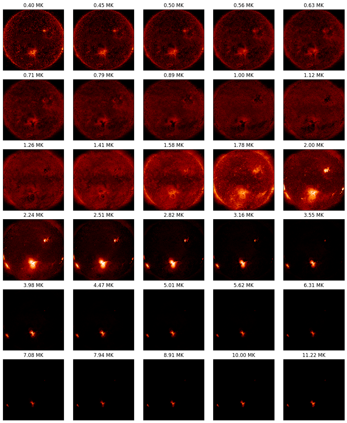
[8]:
fig = plt.figure(figsize=(15,15*6/5))
norm = ImageNormalize(vmin=1e23,vmax=1e28, stretch=LogStretch())
tbin_centers = dem_cube.axis_world_coords(0)[0].to('MK')
for i in range(dem_cube.data.shape[0]):
    ax = fig.add_subplot(6,5,i+1,projection=dem_cube[i].wcs)
    dem_cube[i].plot(axes=ax, norm=norm, cmap='hinodexrt')
    lon,lat = ax.coords
    lon.set_ticklabel_visible(False)
    lat.set_ticklabel_visible(False)
    lon.set_ticks_visible(False)
    lat.set_ticks_visible(False)
    ax.set_title(f'{tbin_centers[i]:.2f}')
plt.subplots_adjust(hspace=0.15,wspace=0.1)
2. Read in CHIANTI Spectra#
[9]:
spectral_table = read_spectral_table('spectral-table.asdf')
WARNING: UnitsWarning: The unit 'Angstrom' has been deprecated in the VOUnit standard. Suggested: 0.1nm. [astropy.units.format.utils]
WARNING: AstropyDeprecationWarning: The truth value of a Quantity is ambiguous. In the future this will raise a ValueError. [astropy.units.quantity]
[10]:
fig = plt.figure(figsize=(15,5))
spectral_table.plot(aspect=20,
                    axes_units=('MK','Angstrom'),
                    norm=ImageNormalize(stretch=LogStretch()),
                    cmap='plasma')
plt.colorbar(label=spectral_table.unit)
plt.title('Feldman CHIANTI Spectra')
WARNING: UnitsWarning: The unit 'Angstrom' has been deprecated in the VOUnit standard. Suggested: 0.1nm. [astropy.units.format.utils]
[10]:
Text(0.5, 1.0, 'Feldman CHIANTI Spectra')

[11]:
fig = plt.figure(figsize=(15,5))
i_T = np.argmin(np.fabs(spectral_table.axis_world_coords(0)[0] - 10**6.4*u.K))
ax = spectral_table[i_T,:].plot()
WARNING: UnitsWarning: The unit 'Angstrom' has been deprecated in the VOUnit standard. Suggested: 0.1nm. [astropy.units.format.utils]
WARNING: UnitsWarning: The unit 'Angstrom' has been deprecated in the VOUnit standard. Suggested: 0.1nm. [astropy.units.format.utils]

Let’s zoom in on the brightest line near 18.9 Å
[12]:
fig = plt.figure(figsize=(15,5))
i_T = np.argmin(np.fabs(spectral_table.axis_world_coords(0)[0] - 10**6.4*u.K))
ax = spectral_table[i_T,:].plot()
ax.set_xlim(spectral_table[i_T,:].wcs.world_to_pixel([18.5,19.5]*u.angstrom))
WARNING: UnitsWarning: The unit 'Angstrom' has been deprecated in the VOUnit standard. Suggested: 0.1nm. [astropy.units.format.utils]
WARNING: UnitsWarning: The unit 'Angstrom' has been deprecated in the VOUnit standard. Suggested: 0.1nm. [astropy.units.format.utils]
[12]:
(318.1818213344431, 336.36364266888614)

3. Integrate EM over temperature#
Now, we compute the spectral cube by integrating each spectra over temperature, weighted by the emission measure distribution.
[13]:
spec_cube = InstrumentDEM.calculate_intensity(
    dem_cube,
    spectral_table,
    dict(celestial_wcs.to_header())
)
WARNING: UnitsWarning: The unit 'Angstrom' has been deprecated in the VOUnit standard. Suggested: 0.1nm. [astropy.units.format.utils]
Let’s pick out the brightest pixel of the cube summed in wavelength and then plot the spectrum for that pixel.
[14]:
ymax,xmax = np.unravel_index(np.argmax(spec_cube.data.sum(axis=0)),spec_cube.data.shape[1:])
[15]:
ax = spec_cube[:,ymax,xmax].plot(axes_units=['Angstrom'],
                                 data_unit='ph /(cm2 Angstrom s sr)')
ax.coords[0].set_major_formatter('x.x')
#plt.yscale('log')
#plt.ylim(1e10,1e15)

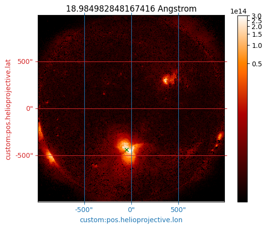
Let’s plot the image corresponding to the brightest line in the above spectra. I’ve marked the corresponding coordinate of maximum intensity with a green x.
[16]:
wave_index = np.argmax(spec_cube[:,ymax,xmax].data)
wave0 = spec_cube.axis_world_coords(0)[0][np.argmax(spec_cube[:,ymax,xmax].data)]
print(wave0.to('Angstrom'))
18.984982848167416 Angstrom
[21]:
norm = ImageNormalize(vmin=1,vmax=3e14, stretch=LogStretch())
fig = plt.figure(figsize=(7,5))
ax = fig.add_subplot(111, projection=spec_cube[wave_index])
spec_cube[wave_index].plot(
    axes=ax,
    cmap='hinodexrt',
    norm=norm,
    data_unit='ph / (cm2 Angstrom s sr)'
)
color_lat_lon_axes(ax)
ax.set_title(spec_cube.axis_world_coords(0)[0][wave_index].to('Angstrom'))
ax.plot(xmax,ymax,ls='',marker='x',color='g')
plt.colorbar()
[21]:
<matplotlib.colorbar.Colorbar at 0x14acb2a30>
4. Fold in instrument response#
Next, fold this cube through the instrument response. This multiplies by the effective area, spatial plate scale, and spectral plate scale. We’ll do this just for the 1st order case.
[22]:
chan = SpectrogramChannel(1, '../../mocksipipeline/data/MOXSI_effarea.genx')
First, take a look at the effective area curve
[23]:
with quantity_support():
    plt.plot(chan.wavelength, chan.effective_area)

As well as the plate scale values
[24]:
print(chan.plate_scale)
7.529785349783243e-10 sr / pix
[25]:
print(chan.spectral_resolution)
0.055 Angstrom / pix
Let’s convolve the spectral cube and the response
[26]:
instr_cube = convolve_with_response(spec_cube, chan, include_gain=False)
And plot the two at the same wavelength as before
[27]:
wave_index = np.argmin(np.fabs(wave0 - instr_cube.axis_world_coords(0)[0]))
WARNING: UnitsWarning: The unit 'Angstrom' has been deprecated in the VOUnit standard. Suggested: 0.1nm. [astropy.units.format.utils]
[29]:
norm = ImageNormalize(vmin=0.01,vmax=300, stretch=LogStretch())
fig = plt.figure(figsize=(7,5))
ax = fig.add_subplot(111, projection=instr_cube[wave_index])
instr_cube[wave_index].plot(
    axes=ax,
    cmap='hinodexrt',
    norm=norm,
    data_unit='ph / (Angstrom pix h)'
)
color_lat_lon_axes(ax)
ax.set_title(instr_cube.axis_world_coords(0)[0][wave_index].to('Angstrom'))
#ax.plot(xmax,ymax,ls='',marker='x',color='g')
plt.colorbar()
WARNING: UnitsWarning: The unit 'Angstrom' has been deprecated in the VOUnit standard. Suggested: 0.1nm. [astropy.units.format.utils]
WARNING: UnitsWarning: The unit 'Angstrom' has been deprecated in the VOUnit standard. Suggested: 0.1nm. [astropy.units.format.utils]
[29]:
<matplotlib.colorbar.Colorbar at 0x14b00c7c0>

[30]:
ymax,xmax = np.unravel_index(np.argmax(instr_cube.data.sum(axis=0)),
                             instr_cube.data.shape[1:])
[32]:
ax = instr_cube[:,ymax,xmax].plot(axes_units=['Angstrom'],
                                  data_unit='ph /(Angstrom pix h)')
ax.coords[0].set_major_formatter('x.x')
#plt.yscale('log')
#plt.ylim(1e10,1e15)
WARNING: UnitsWarning: The unit 'Angstrom' has been deprecated in the VOUnit standard. Suggested: 0.1nm. [astropy.units.format.utils]
WARNING: UnitsWarning: The unit 'Angstrom' has been deprecated in the VOUnit standard. Suggested: 0.1nm. [astropy.units.format.utils]

5. Reproject to Detector Plane#
[35]:
client = distributed.Client()
2022-09-16 12:56:06,665 - distributed.diskutils - INFO - Found stale lock file and directory '/var/folders/cr/pj7yk8p976d7ny98bgvlpfyr0000gq/T/dask-worker-space/worker-zh6drz_1', purging
2022-09-16 12:56:06,666 - distributed.diskutils - INFO - Found stale lock file and directory '/var/folders/cr/pj7yk8p976d7ny98bgvlpfyr0000gq/T/dask-worker-space/worker-1__egu2v', purging
2022-09-16 12:56:06,666 - distributed.diskutils - INFO - Found stale lock file and directory '/var/folders/cr/pj7yk8p976d7ny98bgvlpfyr0000gq/T/dask-worker-space/worker-ae3ezdc9', purging
2022-09-16 12:56:06,666 - distributed.diskutils - INFO - Found stale lock file and directory '/var/folders/cr/pj7yk8p976d7ny98bgvlpfyr0000gq/T/dask-worker-space/worker-wf841za5', purging
2022-09-16 12:56:06,667 - distributed.diskutils - INFO - Found stale lock file and directory '/var/folders/cr/pj7yk8p976d7ny98bgvlpfyr0000gq/T/dask-worker-space/worker-zivsrz0g', purging
[38]:
overlap_o1 = reproject_to_overlappogram(
    instr_cube,
    chan.detector_shape,
    observer=observer,
    reference_pixel=(
        (chan.detector_shape[1] + 1)/2,
        (chan.detector_shape[0] + 1)/2,
        1,
    ) * u.pix,
    reference_coord=(
        0 * u.arcsec,
        0 * u.arcsec,
        chan.wavelength[0],
    ),
    scale=(
        chan.resolution[0],
        chan.resolution[1],
        chan.spectral_resolution,
    ),
    roll_angle=-90*u.deg,
    dispersion_angle=0*u.deg,
    dispersion_axis=0,
    order=chan.spectral_order,
    meta_keys=['CHANNAME'],
    use_dask=True,
    sum_over_lambda=True,
    algorithm='interpolation',
)
WARNING: UnitsWarning: The unit 'Angstrom' has been deprecated in the VOUnit standard. Suggested: 0.1nm. [astropy.units.format.utils]
WARNING: FITSFixedWarning: 'datfix' made the change 'Set MJD-OBS to 59162.750077 from DATE-OBS'. [astropy.wcs.wcs]
WARNING: No observer defined on WCS, SpectralCoord will be converted without any velocity frame change [astropy.wcs.wcsapi.fitswcs]
WARNING: No observer defined on WCS, SpectralCoord will be converted without any velocity frame change [astropy.wcs.wcsapi.fitswcs]
WARNING: No observer defined on WCS, SpectralCoord will be converted without any velocity frame change [astropy.wcs.wcsapi.fitswcs]
WARNING: No observer defined on WCS, SpectralCoord will be converted without any velocity frame change [astropy.wcs.wcsapi.fitswcs]
WARNING: No observer defined on WCS, SpectralCoord will be converted without any velocity frame change [astropy.wcs.wcsapi.fitswcs]
Now, analyze the resulting overlappogram
[39]:
hpc_frame = astropy.wcs.utils.wcs_to_celestial_frame(overlap_o1.wcs)
blc = SkyCoord(Tx=-275*u.arcsec, Ty=-650*u.arcsec, frame=hpc_frame)
trc = SkyCoord(Tx=275*u.arcsec, Ty=5600*u.arcsec, frame=hpc_frame)
lower = SkyCoord(Tx=[trc.Tx,trc.Tx],Ty=[blc.Ty,trc.Ty],frame=hpc_frame)
upper = SkyCoord(Tx=[blc.Tx,blc.Tx],Ty=[blc.Ty,trc.Ty],frame=hpc_frame)
[43]:
fig = plt.figure(figsize=(15,5))
wave_index = 0
norm = ImageNormalize(vmin=0,vmax=300,stretch=LogStretch())
ax = fig.add_subplot(111, projection=overlap_o1[wave_index].wcs)
plot_unit = 'ph / (Angstrom pix h)'
overlap_o1[wave_index].plot(
    axes=ax,
    cmap='hinodexrt',
    norm=norm,
    data_unit=plot_unit
)
ax.plot_coord(lower, ls='--', color='w', lw=2)
ax.plot_coord(upper, ls='--', color='w', lw=2)
im = ax.get_images()[0]
divider = make_axes_locatable(ax)
cax = divider.append_axes('right', size='2%', pad=0.05, axes_class=matplotlib.axes.Axes)
cbar = fig.colorbar(im, cax=cax, orientation='vertical')
cax.yaxis.set_ticks_position("right")
cbar.set_label(f'{plot_unit}',)
color_lat_lon_axes(ax)
[43]:
(<astropy.visualization.wcsaxes.coordinate_helpers.CoordinateHelper at 0x15270f970>,
 <astropy.visualization.wcsaxes.coordinate_helpers.CoordinateHelper at 0x1524cceb0>)

[44]:
overlap_o1_crop = overlap_o1[wave_index].crop(blc, trc)
[45]:
fig = plt.figure(figsize=(15,2.5))
ax = fig.add_subplot(111, projection=overlap_o1_crop.wcs)
overlap_o1_crop.plot(
    axes=ax,
    cmap='hinodexrt',
    norm=norm,
    data_unit=plot_unit
)
im = ax.get_images()[0]
divider = make_axes_locatable(ax)
cax = divider.append_axes('right', size='2%', pad=0.05, axes_class=matplotlib.axes.Axes)
cbar = fig.colorbar(im, cax=cax, orientation='vertical')
cax.yaxis.set_ticks_position("right")
cbar.set_label(f'{plot_unit}',)
color_lat_lon_axes(ax)
[45]:
(<astropy.visualization.wcsaxes.coordinate_helpers.CoordinateHelper at 0x151f7eeb0>,
 <astropy.visualization.wcsaxes.coordinate_helpers.CoordinateHelper at 0x151ddfa30>)

[46]:
pix_x_cut = np.linspace(0, overlap_o1_crop.data.shape[1]-1, overlap_o1_crop.data.shape[1])
coord_cut = overlap_o1_crop.wcs.pixel_to_world(pix_x_cut, (overlap_o1_crop.data.shape[0]-1)/2)
[51]:
ar_sum = u.Quantity(overlap_o1_crop.data.sum(axis=0), overlap_o1_crop.unit)

fig = plt.figure(figsize=(8,5))
ax = fig.add_subplot(111)
with quantity_support():
    ax.plot(coord_cut.Ty, ar_sum.to(plot_unit),)
ax.set_yscale('log')
ax.set_ylim(1,1e5)
ax.set_xlim(coord_cut.Ty[[0,-1]].to_value('arcsec'))
[51]:
(-648.0678674871172, 5599.194270288217)

Sandbox#
[12]:
import specutils
from specutils.manipulation import FluxConservingResampler, LinearInterpolatedResampler
[13]:
spectral_table
[13]:
<ndcube.ndcube.NDCube object at 0x14e9d6fa0>
NDCube
------
Dimensions: [  21. 1073.] pix
Physical Types of Axes: [('phys.temperature', 'phys.density'), ('em.wl',)]
Unit: cm3 ph / (Angstrom s sr)
Data Type: float64
[14]:
su_spec_cube = specutils.Spectrum1D(flux=spectral_table.data*spectral_table.unit, wcs=spectral_table[0,:].wcs)
[15]:
su_spec_cube
[15]:
<Spectrum1D(flux=<Quantity [[2.25204783e-211, 4.31376155e-201, 7.89238649e-192, ...,
            4.23137487e-019, 4.25571018e-019, 4.28017755e-019],
           [7.68563820e-171, 1.12038522e-162, 2.52956409e-155, ...,
            1.05246430e-018, 1.05688938e-018, 1.06146775e-018],
           [1.21703856e-138, 3.68088464e-132, 2.53135171e-126, ...,
            1.93597584e-018, 1.94111890e-018, 1.94851103e-018],
           ...,
           [2.74227206e-019, 3.81211277e-019, 5.11706501e-019, ...,
            7.63286147e-018, 7.62821787e-018, 7.62608485e-018],
           [9.59901649e-019, 1.23590792e-018, 1.54836156e-018, ...,
            7.31056620e-018, 7.30593205e-018, 7.30136578e-018],
           [2.57148386e-018, 3.11639307e-018, 3.69725574e-018, ...,
            6.97364966e-018, 6.96899607e-018, 6.96435276e-018]] cm3 ph / (Angstrom s sr)>, spectral_axis=<SpectralAxis [ 1.        ,  1.05499995,  1.11000001, ..., 59.84999847, 59.90499878,
   59.95999908] Angstrom>)>
[41]:
new_spec_axis = np.arange(*su_spec_cube.spectral_axis[[0,-1]].to_value('Angstrom'),
                          0.01) * u.Angstrom
[42]:
fcon_interp = FluxConservingResampler()
[43]:
new_su_spec_cube = fcon_interp(su_spec_cube, new_spec_axis.to(su_spec_cube.spectral_axis.unit))
[44]:
plt.figure(figsize=(15,8))
plt.step(su_spec_cube.spectral_axis, su_spec_cube.data[9,:])
plt.step(new_su_spec_cube.spectral_axis, new_su_spec_cube.data[9,:])
plt.xlim(15,20)
#plt.yscale('log')
[44]:
(15.0, 20.0)

[69]:
su_spec_cube.spectral_axis_unit
WARNING: AstropyDeprecationWarning: The spectral_axis_unit function is deprecated and may be removed in a future version.
        Use spectral_axis.unit instead. [warnings]
[69]:
[ ]: