[2]:
import xarray
import numpy as np
from sklearn.linear_model import ElasticNet, LassoLars, ElasticNetCV
from sklearn.pipeline import make_pipeline
from sklearn.preprocessing import StandardScaler
import matplotlib.pyplot as plt
from astropy.visualization import ImageNormalize, LogStretch, AsinhStretch

%matplotlib inline
Inversion Tests#
Some tests to see how easy it is to invert the MOXSI data
Load the response matrix and EM cube
[3]:
response_matrix = xarray.open_dataarray('moxsi_response_matrix.nc')
[4]:
response_matrix_total = response_matrix.sum(dim='spectral_order').rename({'pixel_fov': 'pixel_x'})
[5]:
response_matrix_total
[5]:
<xarray.DataArray (pixel_x: 338, pixel_detector: 2000, log_temperature: 60)>
array([[[5.47814223e-40, 3.69993772e-39, 1.94958896e-38, ...,
         3.54270315e-33, 3.46808906e-33, 3.39052206e-33],
        [5.37407903e-40, 3.64142754e-39, 1.92480694e-38, ...,
         3.57883643e-33, 3.50438533e-33, 3.42679047e-33],
        [5.27135532e-40, 3.58307651e-39, 1.89881003e-38, ...,
         3.64502537e-33, 3.56380521e-33, 3.48082210e-33],
        ...,
        [1.73253895e-38, 5.44433530e-38, 1.44729630e-37, ...,
         3.76546405e-34, 3.67455789e-34, 3.58322216e-34],
        [1.73662874e-38, 5.44834886e-38, 1.44631722e-37, ...,
         3.67828793e-34, 3.59475551e-34, 3.50992945e-34],
        [1.74064531e-38, 5.45209437e-38, 1.44523028e-37, ...,
         3.64191502e-34, 3.55908754e-34, 3.47494412e-34]],

       [[5.58397589e-40, 3.75944844e-39, 1.97535564e-38, ...,
         3.50856419e-33, 3.43412174e-33, 3.35698097e-33],
        [5.47814223e-40, 3.69993772e-39, 1.94958896e-38, ...,
         3.54270315e-33, 3.46808906e-33, 3.39052206e-33],
        [5.37407903e-40, 3.64142754e-39, 1.92480694e-38, ...,
         3.57883643e-33, 3.50438533e-33, 3.42679047e-33],
...
        [5.37407903e-40, 3.64142754e-39, 1.92480694e-38, ...,
         3.57883643e-33, 3.50438533e-33, 3.42679047e-33],
        [5.47814223e-40, 3.69993772e-39, 1.94958896e-38, ...,
         3.54270315e-33, 3.46808906e-33, 3.39052206e-33],
        [5.58397589e-40, 3.75944844e-39, 1.97535564e-38, ...,
         3.50856419e-33, 3.43412174e-33, 3.35698097e-33]],

       [[1.74064531e-38, 5.45209437e-38, 1.44523028e-37, ...,
         3.64191502e-34, 3.55908754e-34, 3.47494412e-34],
        [1.73662874e-38, 5.44834886e-38, 1.44631722e-37, ...,
         3.67828793e-34, 3.59475551e-34, 3.50992945e-34],
        [1.73253895e-38, 5.44433530e-38, 1.44729630e-37, ...,
         3.76546405e-34, 3.67455789e-34, 3.58322216e-34],
        ...,
        [5.27135532e-40, 3.58307651e-39, 1.89881003e-38, ...,
         3.64502537e-33, 3.56380521e-33, 3.48082210e-33],
        [5.37407903e-40, 3.64142754e-39, 1.92480694e-38, ...,
         3.57883643e-33, 3.50438533e-33, 3.42679047e-33],
        [5.47814223e-40, 3.69993772e-39, 1.94958896e-38, ...,
         3.54270315e-33, 3.46808906e-33, 3.39052206e-33]]])
Coordinates:
  * log_temperature  (log_temperature) float64 5.0 5.05 5.1 ... 7.85 7.9 7.95
Dimensions without coordinates: pixel_x, pixel_detector1. Observed EM#
Create simulated MOXSI data
[6]:
em_cube_observed = xarray.open_dataarray('observed-dem.nc')
[7]:
moxsi_counts_observed = response_matrix_total.dot(em_cube_observed, dims=['log_temperature', 'pixel_x']).T
[9]:
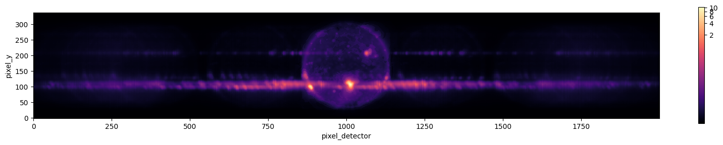
fig = plt.figure(figsize=(20,3))
ax = fig.add_subplot()
moxsi_counts_observed.plot.imshow(ax=ax, cmap='magma', norm=ImageNormalize(stretch=LogStretch()), interpolation='none')
ax.set_aspect(1)
[10]:
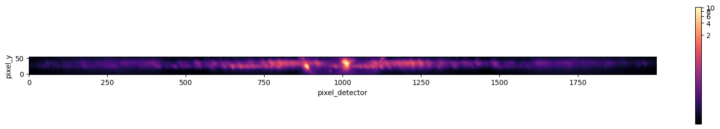
fig = plt.figure(figsize=(20,3))
ax = fig.add_subplot()
moxsi_counts_observed[75:130,:].plot.imshow(ax=ax, cmap='magma', norm=ImageNormalize(stretch=LogStretch()), interpolation='none')
ax.set_aspect(1)
[12]:
fig = plt.figure(figsize=(20,8))
moxsi_counts_observed[75:130,:].sum(dim='pixel_y').plot()
plt.yscale('log')
#plt.ylim(1e-4,1)

[229]:
moxsi_counts_observed
[229]:
<xarray.DataArray (pixel_y: 338, pixel_detector: 2000)>
array([[8.88842748e-06, 8.26483954e-06, 9.25301489e-06, ...,
        8.91252732e-06, 8.67358830e-06, 8.86702947e-06],
       [9.92176314e-06, 9.25198295e-06, 1.01512446e-05, ...,
        9.55712933e-06, 9.63087563e-06, 9.71864626e-06],
       [1.16514876e-05, 1.11142538e-05, 1.17011280e-05, ...,
        1.09602735e-05, 1.11107251e-05, 1.10209396e-05],
       ...,
       [1.38433505e-05, 1.33900401e-05, 1.41949669e-05, ...,
        1.39063150e-05, 1.42248696e-05, 1.40559468e-05],
       [1.26016401e-05, 1.21549025e-05, 1.30693955e-05, ...,
        1.26190121e-05, 1.27588297e-05, 1.26152542e-05],
       [1.13154978e-05, 1.06820666e-05, 1.18868067e-05, ...,
        1.10680595e-05, 1.09213840e-05, 1.10947184e-05]])
Dimensions without coordinates: pixel_y, pixel_detectorNow, try to do an actual inversion
[15]:
x_ = response_matrix_total.stack(pixel_logT=('pixel_x', 'log_temperature'))
[16]:
SCALING_CONSTANT = 1e30
[19]:
#pipeline = make_pipeline(
#    StandardScaler(),
#    #ElasticNet(),
#    LassoLars()
#)
#model = LassoLars(verbose=1, alpha=1.5, positive=True, max_iter=1000)
#model = ElasticNetCV(
#    positive=True,
#    alphas=[1.5,],
#    l1_ratio=[.9e-5, 1e-4, 5e-4, 7.5e-4],
#    max_iter=2000,
#    n_jobs=-1,
#)
model = ElasticNet(
    positive=True,
    alpha=1.1,
    l1_ratio=1e-4,
    max_iter=2000,
)
[20]:
model.fit(x_.values*SCALING_CONSTANT, moxsi_counts_observed[100,:].values, )
[20]:
ElasticNet(alpha=1.1, l1_ratio=0.0001, max_iter=2000, positive=True)In a Jupyter environment, please rerun this cell to show the HTML representation or trust the notebook.
On GitHub, the HTML representation is unable to render, please try loading this page with nbviewer.org.
ElasticNet(alpha=1.1, l1_ratio=0.0001, max_iter=2000, positive=True)
[22]:
em_coefficients = xarray.DataArray(
    model.coef_,
    dims=['pixel_logT'],
    coords={'pixel_logT': x_.pixel_logT},
)*SCALING_CONSTANT
[23]:
recovered_moxsi_counts_observed = x_.dot(em_coefficients, dims=['pixel_logT'])
[25]:
plt.figure(figsize=(25,5))
recovered_moxsi_counts_observed.plot(label='recovered')
moxsi_counts_observed[100,:].plot(label='data')
plt.yscale('log')
plt.legend()
[25]:
<matplotlib.legend.Legend at 0x3fe7f3c70>

[26]:
em_recovered_observed = em_coefficients.unstack()
[31]:
norm = ImageNormalize(vmin=1e23, vmax=1e27, stretch=LogStretch())
plt.figure(figsize=(12,6))
plt.subplot(121)
em_recovered_observed.plot(norm=norm)
plt.subplot(122)
em_cube_observed[100,...].plot(norm=norm)
[31]:
<matplotlib.collections.QuadMesh at 0x3ffb1aa90>

[32]:
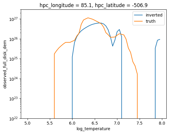
em_recovered_observed.isel(pixel_x=180).plot(label='inverted')
em_cube_observed.isel(pixel_y=100, pixel_x=180).plot(label='truth')
plt.yscale('log')
plt.ylim(1e22,3e27)
plt.legend()
[32]:
<matplotlib.legend.Legend at 0x40004cf40>
2. Simulated EM#
[50]:
em_cube_simulated = xarray.open_dataarray('simulated-dem.nc')[78:144,150:204,...]
[51]:
em_cube_simulated
[51]:
<xarray.DataArray 'simulated_dem' (pixel_y: 66, pixel_x: 54, log_temperature: 60)>
[213840 values with dtype=float64]
Coordinates:
    hpc_longitude    (pixel_y, pixel_x) float64 -136.9 -129.5 ... 247.9 255.3
    hpc_latitude     (pixel_y, pixel_x) float64 -669.7 -669.7 ... -188.7 -188.7
  * log_temperature  (log_temperature) float64 5.0 5.05 5.1 ... 7.85 7.9 7.95
Dimensions without coordinates: pixel_y, pixel_x
Attributes:
    bunit:     cm-5
    wcsaxes:   2
    crpix1:    169.5
    crpix2:    169.5
    cdelt1:    0.0020555555555556
    cdelt2:    0.0020555555555556
    cunit1:    deg
    cunit2:    deg
    ctype1:    HPLN-TAN
    ctype2:    HPLT-TAN
    crval1:    0.0
    crval2:    0.0
    lonpole:   180.0
    latpole:   0.0
    mjdref:    0.0
    date-obs:  2020-11-09T17:59:57.340
    mjd-obs:   59162.749969213
    rsun_ref:  696000000.0
    dsun_obs:  148154617444.64
    hgln_obs:  0.0
hglt_obs: 3.4233542990553[52]:
moxsi_counts_simulated = response_matrix_total[150:204,...].dot(em_cube_simulated, dims=['log_temperature', 'pixel_x']).T
[53]:
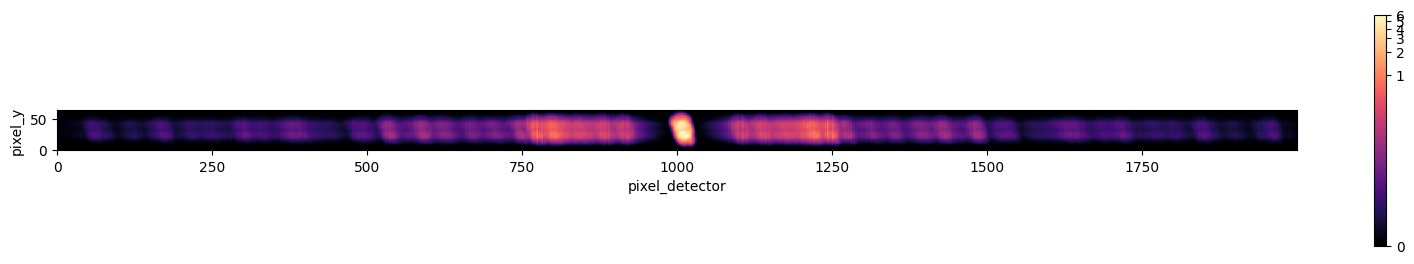
fig = plt.figure(figsize=(20,3))
ax = fig.add_subplot()
moxsi_counts_simulated.plot.imshow(ax=ax, cmap='magma', norm=ImageNormalize(stretch=LogStretch()), interpolation='none')
ax.set_aspect(1)
[208]:
fig = plt.figure(figsize=(20,8))
moxsi_counts_simulated.sum(dim='pixel_y').plot(label='total')
moxsi_counts_simulated.isel(pixel_y=30).plot(label='pixel_y=30')
moxsi_counts_simulated.isel(pixel_y=45).plot(label='pixel_y=45')
plt.yscale('log')
#plt.ylim(1e-4,1)
plt.legend()
[208]:
<matplotlib.legend.Legend at 0x467647130>

[209]:
x_ = response_matrix_total[150:204,...].stack(pixel_logT=('pixel_x', 'log_temperature'))
[210]:
model = ElasticNet(
    positive=True,
    alpha=0.05,
    l1_ratio=2.5e-5,
    max_iter=2000,
    fit_intercept=False,
)
[211]:
model.fit(x_.values*SCALING_CONSTANT, moxsi_counts_simulated[40,:].values, )
[211]:
ElasticNet(alpha=0.05, fit_intercept=False, l1_ratio=2.5e-05, max_iter=2000,
           positive=True)
In a Jupyter environment, please rerun this cell to show the HTML representation or trust the notebook. On GitHub, the HTML representation is unable to render, please try loading this page with nbviewer.org.
ElasticNet(alpha=0.05, fit_intercept=False, l1_ratio=2.5e-05, max_iter=2000,
           positive=True)
[212]:
em_coefficients = xarray.DataArray(
    model.coef_,
    dims=['pixel_logT'],
    coords={'pixel_logT': x_.pixel_logT},
)*SCALING_CONSTANT
[213]:
recovered_moxsi_counts_simulated = x_.dot(em_coefficients, dims=['pixel_logT'])
[214]:
plt.figure(figsize=(25,5))
recovered_moxsi_counts_simulated.plot(label='recovered')
moxsi_counts_simulated[40,:].plot(label='data')
plt.yscale('log')
plt.legend()
[214]:
<matplotlib.legend.Legend at 0x46763ab20>

[215]:
em_recovered_simulated = em_coefficients.unstack()
[216]:
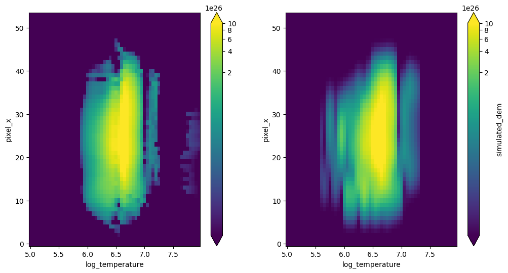
norm = ImageNormalize(vmin=1e23, vmax=1e27, stretch=LogStretch())
plt.figure(figsize=(12,6))
plt.subplot(121)
em_recovered_simulated.plot(norm=norm)
plt.subplot(122)
em_cube_simulated[40,...].plot(norm=norm)
[216]:
<matplotlib.collections.QuadMesh at 0x47b3535b0>
[227]:
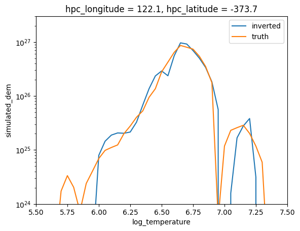
em_recovered_simulated.isel(pixel_x=35).plot(label='inverted')
em_cube_simulated.isel(pixel_y=40, pixel_x=35).plot(label='truth')
plt.yscale('log')
plt.ylim(1e24,3e27)
plt.xlim(5.5,7.5)
plt.legend()
[227]:
<matplotlib.legend.Legend at 0x47da9b610>
[ ]:
foo = np.random.rand(10,50,30)
[ ]:
foo_idx = np.where(foo > 0.5)
[201]:
foo_idx
[201]:
(array([0, 0, 0, ..., 9, 9, 9]),
 array([ 0,  0,  0, ..., 49, 49, 49]),
 array([ 0,  1,  2, ..., 23, 25, 28]))
[202]:
def print_index(iz,iy,ix):
    print(iz)
    print(iy)
    print(ix)
[204]:
print_index(*foo_idx)
[0 0 0 ... 9 9 9]
[ 0  0  0 ... 49 49 49]
[ 0  1  2 ... 23 25 28]
[205]:
print_index(*foo_idx[::-1])
[ 0  1  2 ... 23 25 28]
[ 0  0  0 ... 49 49 49]
[0 0 0 ... 9 9 9]
[ ]: