[5]:
import itertools

import astropy.units as u
import numpy as np
import astropy.time
import matplotlib.pyplot as plt
from astropy.visualization import quantity_support
import astropy.constants as const
import sunpy.map

import xrtpy
import aiapy.response
[6]:
mxrt = sunpy.map.Map('/Users/wtbarnes/sunpy/data/comp_XRT20201109_053212.9.fits')
[12]:
mxrt.meta['TELESCOP']
[12]:
'HINODE'
[13]:
mxrt.measurement
[13]:
'Open-Al mesh'
[2]:
from xrtpy.response.effective_area import index_mapping_to_fw1_name, index_mapping_to_fw2_name
[3]:
index_mapping_to_fw1_name
[3]:
{'Open': 0, 'Al-poly': 1, 'C-poly': 2, 'Be-thin': 3, 'Be-med': 4, 'Al-med': 5}
[4]:
index_mapping_to_fw2_name
[4]:
{'Open': 0,
 'Al-mesh': 1,
 'Ti-poly': 2,
 'G-band': 3,
 'Al-thick': 4,
 'Be-thick': 5}
[7]:
filters = [
    'Al-poly',
    'Be-thin',
    'Be-med',
    'Be-thick',
]
date = astropy.time.Time('2006-09-22T22:00:00')
Temperature Response Functions#
[27]:
foo = xrtpy.response.TemperatureResponseFundamental('be-thin', date)
[28]:
foo.effective_area() * foo.solid_angle_per_pixel * (const.c * const.h / foo.channel_wavelength).to('eV ph-1') / foo.ev_per_electron / foo.ccd_gain_right
[28]:
$[3.9786996 \times 10^{-19},~1.0326046 \times 10^{-18},~2.4608291 \times 10^{-18},~\dots,~1.5596616 \times 10^{-51},~0,~0] \; \mathrm{\frac{cm^{2}\,DN\,sr}{ph\,pix}}$
[12]:
foo.ev_per_electron
[12]:
$3.6500001 \; \mathrm{\frac{eV}{e^{-}}}$
[13]:
foo.ccd_gain_right
[13]:
$59.099998 \; \mathrm{\frac{e^{-}}{DN}}$
[20]:
foo.channel_wavelength
[20]:
$[1,~1.1,~1.2,~\dots,~399.78699,~399.89301,~400] \; \mathrm{\mathring{A}\,ph}$
[30]:
foo.channel_wavelength
[30]:
$[1,~1.1,~1.2,~\dots,~399.78699,~399.89301,~400] \; \mathrm{\mathring{A}\,ph}$
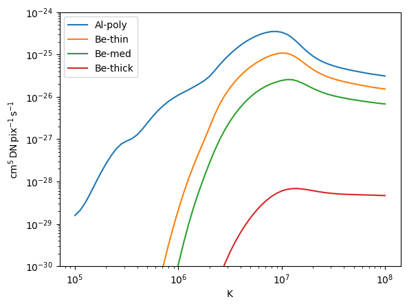
[4]:
temp_response = {}
for f in filters:
    resp = xrtpy.response.TemperatureResponseFundamental(f, date)
    temp_response[resp.name] = (resp.CHIANTI_temperature, resp.temperature_response())
[79]:
with quantity_support():
    for f in temp_response:
        plt.plot(*temp_response[f], label=f)
plt.xscale('log')
plt.yscale('log')
plt.ylim(1e-30,1e-24)
plt.legend()
[79]:
<matplotlib.legend.Legend at 0x17600f400>
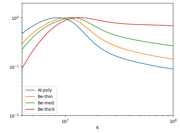
[80]:
with quantity_support():
    for f in temp_response:
        T,tr = temp_response[f]
        plt.plot(T, tr/tr.max(), label=f)
plt.xscale('log')
plt.yscale('log')
plt.ylim(1e-2,2)
plt.xlim(4e6,1e8)
plt.legend()
[80]:
<matplotlib.legend.Legend at 0x29e926af0>
[8]:
pairs = [sorted(p) for p in itertools.product(filters,filters,) if p[0] != p[1]]
pairs = set(['/'.join(p) for p in pairs])
pairs = [p.split('/') for p in pairs]
[109]:
pairs
[109]:
[['Al-poly', 'Be-thick'],
 ['Be-med', 'Be-thin'],
 ['Be-thick', 'Be-thin'],
 ['Be-med', 'Be-thick'],
 ['Al-poly', 'Be-med'],
 ['Al-poly', 'Be-thin']]
[110]:
pairs = [
    ['Al-poly', 'Be-thick'],
    ['Be-thin', 'Be-med'],
    ['Be-thin', 'Be-thick'],
    ['Be-med', 'Be-thick'],
    ['Al-poly', 'Be-med'],
    ['Al-poly', 'Be-thin']
]
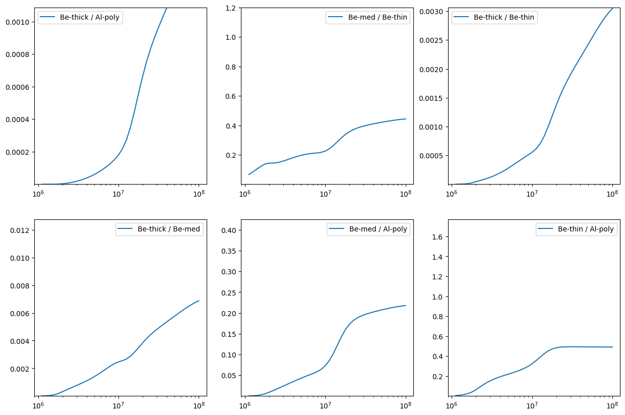
[111]:
fig = plt.figure(figsize=(15,10))
for i,(pa,pb) in enumerate(pairs):
    Ta,tra = temp_response[pa]
    Tb,trb = temp_response[pb]
    i_T = np.where(Ta > 1e6*u.K)
    ratio = trb.to_value('cm5 DN pix-1 s-1')/tra.to_value('cm5 DN pix-1 s-1')
    ratio = ratio[i_T]
    #ratio_grad = np.gradient(ratio, np.gradient(log_T))
    ax = fig.add_subplot(2,3,i+1)
    ax.plot(Ta[i_T], ratio, label=f'{pb} / {pa}')
    ax.set_xscale('log')
    ax.set_ylim(ratio[(ratio.shape[0] + 1)//2]*np.array([0.01,5]))
    ax.legend()
#plt.xlim(1e6,1e8)
#plt.ylim(1e-10,1e10)
#plt.legend(ncol=2)
#plt.axhline(y=1,color='k',ls=':',)
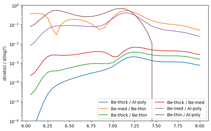
[121]:
fig = plt.figure(figsize=(8,5))
ax = fig.add_subplot(111)
for pa,pb in pairs[:]:
    Ta,tra = temp_response[pa]
    Tb,trb = temp_response[pb]
    i_T = np.where(Ta > 1e6*u.K)
    ratio = trb.to_value('cm5 DN pix-1 s-1')/tra.to_value('cm5 DN pix-1 s-1')
    Ta = Ta[i_T]
    ratio = ratio[i_T]
    log_T = np.log10(Ta.to_value())
    ratio_grad = np.gradient(ratio, log_T)
    ax.plot(log_T, ratio_grad, label=f'{pb} / {pa}')
#ax.set_xscale('log')
#ax.set_yscale('symlog',linthresh=1e-10)
ax.set_yscale('log')
ax.set_ylim(1e-6,1)
ax.set_ylabel('d(ratio) / d(logT)')
ax.legend(ncol=2)
plt.axhline(y=0,color='k',ls=':',)
[121]:
<matplotlib.lines.Line2D at 0x2aadce100>